L12 The Kinetics of Enzymatic Catalysis
一、Michaelis-Menten kinetics
Michaelis-Menten kinetics is about Reaction Rate for a Simple Enzyme-Catalyzed Reaction
The relationship of k’s
An expression for a simple reaction involving a single substrate and product was shown as:

- $k_{1} \text{ and } k_{-1} >> k_{2}$: Binding process is reversible
- $k_{2} >> k_{-2}$: Conversion ES to EP lie far to the right
- $K_{3} >> k_{-2}$: Rapid release of product
If we analyze the initial rate of an enzyme-catalyzed reaction (i.e., before a significant concentration of P appears) and we assume that $k_{1} , k_{-1} \text{ and } k_{3} >> k_{2}$, and Equation 11.12 simplifies to the following:

The catalytic formation of the product, with enzyme regeneration, will then be a simple first-order reaction, and its rate will be determined solely by the concentration of ES and the value of $ k_{cat}$
- 12 公式简化为11.13 公式的形式是在特定假设下的
$k_{cat }$ is the apparent rate constant for the rate-determining conversion of substrate to product
$k_{cat} $ is an aggregate rate constant = $k_{2} k_{3}/(k_{2} + k_{3})$. In the limiting case where $k_{3} >> k_{2}$, $k_{cat} \approx k_{2}$
Initial reaction conditions are such that the reverse reaction between E and P is negligible.
Therefore, the reaction rate, or velocity, defined as the observed rate of formation of products, can be expressed as equation 11.14:
$$
v = k_{cat} [ES]
$$
[ES] is difficult to measure in kinetics experiments. The easily measured parameters are substrate (or product) concentration and the total concentration of enzyme, which must be the sum of free enzyme and enzyme bound to substrate: equation 11.15
$$
[E]{t} = [E] + [ES]
\
\text{Total Enzyme = Free Enzyme + Enzyme in ES complex}
$$
The way we have written Equation 11.13 suggests that E and S should be in equilibrium with ES, with an equilibrium dissociation constant $K{s}$: Equation 11.16
$$
K_{s} = \frac{k_{-1}}{k_{1}} = \frac{[E][S]}{[ES]}
$$
这个对于$K_{s}$的方程式在特定条件下才成立的(This is usually an incorrect assumption, but under certain circumstances ): It doesn’t apply in general because E, S, and ES are not truly in equilibrium
- $k_{cat} << k_{-1}$ this approximation is valid.
Steady State
when the reaction is started by mixing enzymes and substrates, the ES concentration builds up at first, but quickly reaches a steady state, in which it remains almost constant. This steady state will persist until almost all of the substrate has been consumed
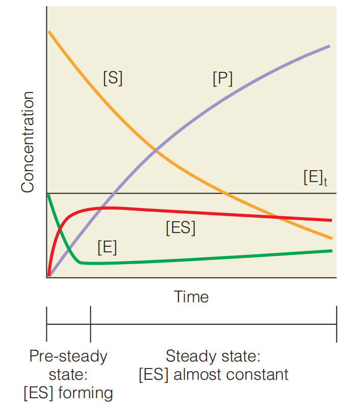
The steady state in enzyme kinetics. The figure shows how the concentrations of substrate [S], free enzyme [E], enzyme–substrate complex [ES], and product [P] vary with time for a simple enzyme-catalyzed reaction
Described by $E + S \rightleftharpoons ES \rarr E + P$ After a very brief initial period, [ES] reaches a steady state in which ES is consumed approximately as rapidly as it is formed, so $d[ES]/dt \approx 0$. The amounts of E and ES are greatly exaggerated for clarity. Note that $[E] + [ES] = [E]_{t}$, or total enzyme concentration, and that [ES] actually falls very slowly as substrate is consumed, while [E] accordingly rises.
In the steady state, the rates of formation and breakdown of ES are equal. Therefore gives equation 11.17
$$
k_{1} [E][S] = k_{-1} [ES] + k_{cat}[ES] \
\text{Formation of ES complex = Disociation of ES complex + Breakdown to E + P}
$$
which can be rearranged to give Equation 11.18
$$
[ES] = (\frac{k_{1}}{k_{-1} + k_{cat}}) [E][S]
$$
Combining the ratio of rate constants in Equation 11.17 gives a single constant, $K_{M}$ equation 11.19
$$
K_{M} = \frac{k_{-1} + k_{cat}}{k_{1}}
$$
Equation 11.18 can now be rewritten as equation 11.20
$$
K_{M} [ES] = [E][S]
$$
At this point, [ES] is expressed in terms of [E] and [S]. To get $[E]{t}$ into the equation, rather than [E], recall from Equation 11.15 that $[E]{t} = [E] + [ES]$ Putting this into Equation 11.20 yields
$$
K_{M} [ES] = [E]{t}[S]-[ES][S]
$$
This rearranges to equation 11.22
$$
[ES] = \frac{[E]{t} [S]}{K_{M} + [S]}
$$
Finally, inserting this result into Equation 11.14 gives an expression for v in terms of $[E]{t} $ and [S]: equation 11.23
$$
v = \frac{k{cat} [E]{t} [S]}{K{M} + [S]}
$$
Michaelis–Menten equation
Equation 11.23 is called the Michaelis–Menten equation, and $K_{M}$ is the Michaelis constant,
- $K_{M}$ is a ratio of the rate constants for a specific reaction (see Equation 11.19), it is a characteristic of that reaction.
- $K_{M}$ has units of concentration.
Velocity
Consider the graph of v versus [S] shown in Figure 11.23.
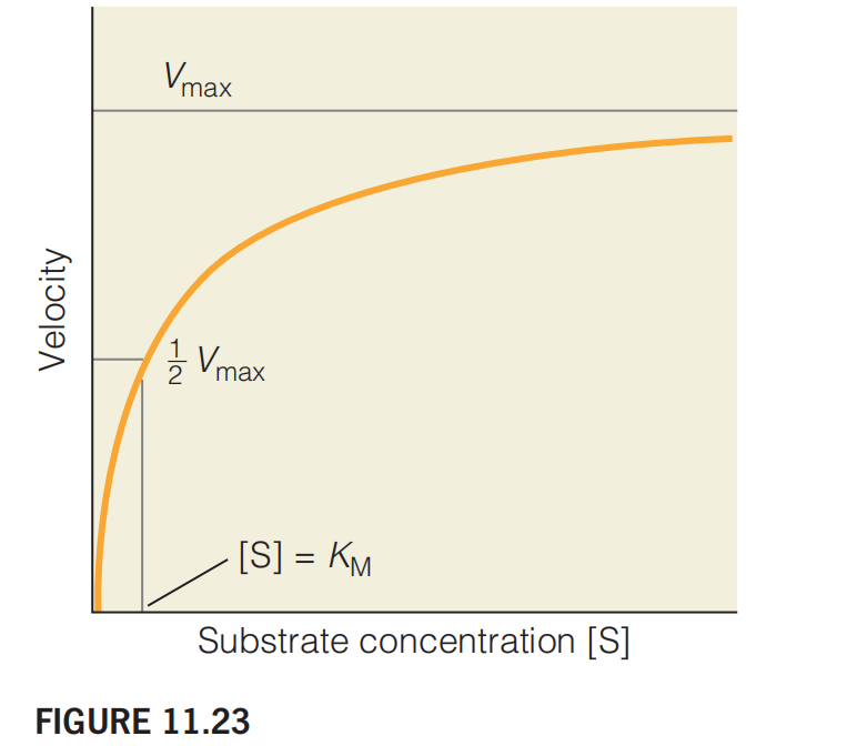
This graph shows the variation of reaction velocity with substrate concentration according to the Michaelis–Menten model of enzyme kinetics.
The values of v plotted here are determined from the initial rates of the reaction.
At the point where [S] = $K_{M }$ the reaction has exactly half its maximum velocity.
Note that $V_{max}$ is approached asymptotically (渐进的).
At high substrate concentrations, where [S] is much greater than $K_{M}$, the reaction approaches a maximum velocity $V_{max}$.
When $[S] >> K_{M}, K_{M} + [S] \approx [S]$, so equation 11.23 can be simplified to equation 11.24 :
$$
V_{max} = k_{cat} [E]{t}
$$
The Michaelis–Menten rate equation is equation 11.25:
$$
v = \frac{V{max} [S]}{K_{M} + [S]}
$$
This is the most familiar form of the Michaelis–Menten equation.
Reaction velocity as a function of substrate concentration. This graph, a plot of Equation 11.25, shows the variation of reaction velocity with substrate concentration according to the Michaelis–Menten model of enzyme kinetics. The values of v plotted here are determined from the initial rates of the reaction (see Figure 11.24). At the point where the reaction has exactly half its maximum velocity. Note that is approached asymptotically.
Significance of $K_{M}$, $k_{cat}$, $V_{max}$
$K_{M} $ is often associated with the affinity of enzyme for substrate.
**However, this relationship is only true in the limiting case: a two-step reaction in which $k_{cat} << k_{1}$**
So equation 11.19 then yields
$$
K_{M} \approx [k_{-1}][k_{1}] = K_{S}
$$
the equilibrium constant defined in Equation 11.16
1. Michaelis constant $K_{M}$
Thus, $K_{M}$ is a measure of the substrate concentration required for effective catalysis to occur.
$K_{M}$ is a equilibrium constant.
An enzyme with a high $K_{M}$ requires a higher substrate concentration to achieve a given reaction velocity than an enzyme with a low $K_{M}$ but the same $k_{cat}$
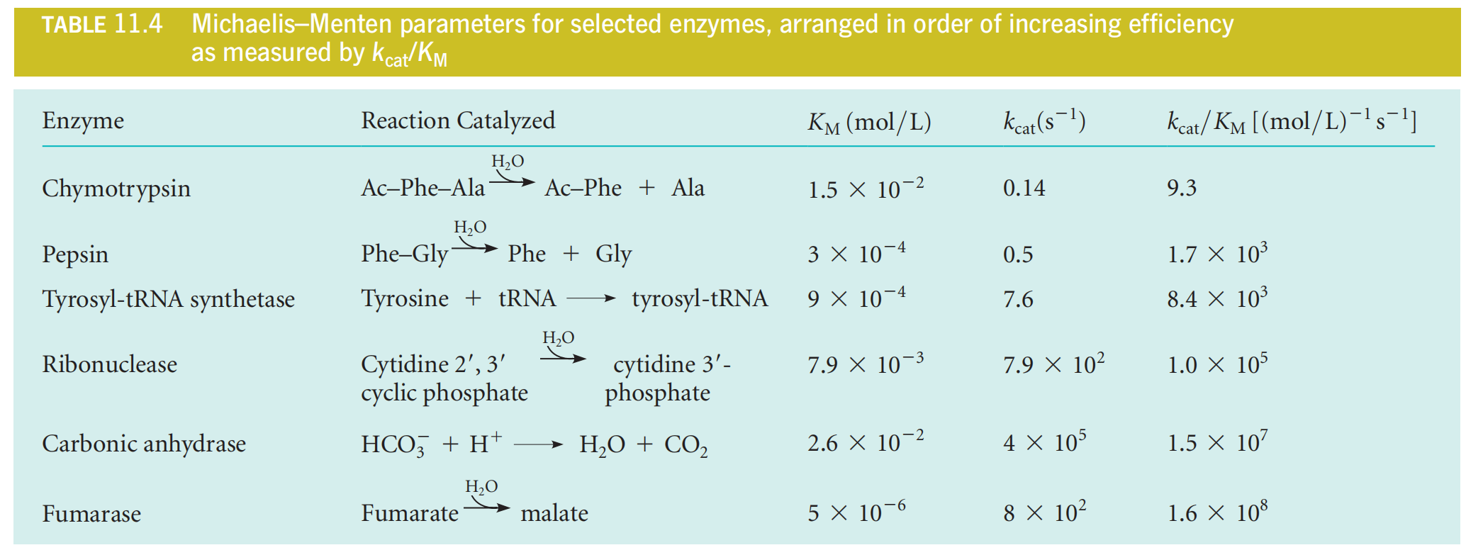
Table 11.4 lists values for a number of important enzymes.
Higher $K_{M}$, the lower ability to bind substrate.
The steady-state assumption proposes that the concentration of enzyme–substrate complex remains nearly constant through much of the reaction.
The Michaelis constant, $K_{M}$ , indicates the substrate concentration at which the reaction rate is ½ Vmax.
2. The Turnover Number $k_{cat}$
The turnover number, $k_{cat} $ , measures the rate of the catalytic process. Some typical turnover numbers are listed in Table 11.4.
$k_{cat}$ is a rate constant.
$k_{cat}$ gives a direct measure of the rate of product formation under optimum conditions (saturated enzyme).
The unit of $k_{cat}$ is always $s^{-1}$
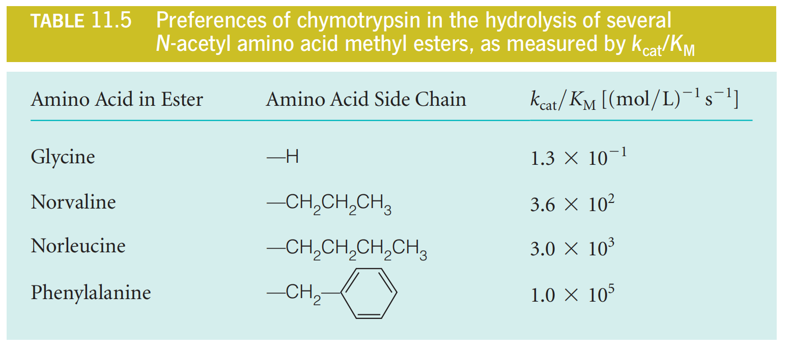
3. The Ratio $k_{cat}/K_{M}$
The ratio $k_{cat}/K_{M}$ is a convenient measure of enzyme efficiency.
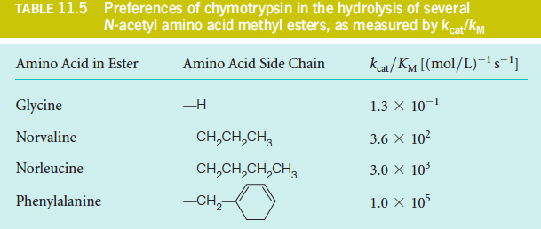
Note that either a large value of $k_{cat}$ (i.e., rapid turnover) or a small value of $K_{M}$ (i.e., $1/2 \ V_{max}$ occurs at relatively low [S]) will make $k_{cat}/K_{M}$ large.
We can gain another insight into the meaning of $k_{cat}/K_{M}$ by considering the situation at very low substrate concentrations.
In this case, $[s] << K_{M}$, so most of the enzyme is free, so $[E]{t} \approx [E]$. Then the equation 11.23 becomes equation 11.26:
$$
v = \frac{k{cat}}{K_{M}} [E][S]
$$
Therefore, under these circumstances, the ratio $k_{cat}/K_{M}$ behaves as a second-order rate constant for the reaction between substrate and free enzyme, and it provides a direct measure of enzyme efficiency and specificity.
Suppose an enzyme has a choice of two substrates, A or B, present at equal concentrations. Then under conditions in which both substrates are dilute and are competing for the enzyme
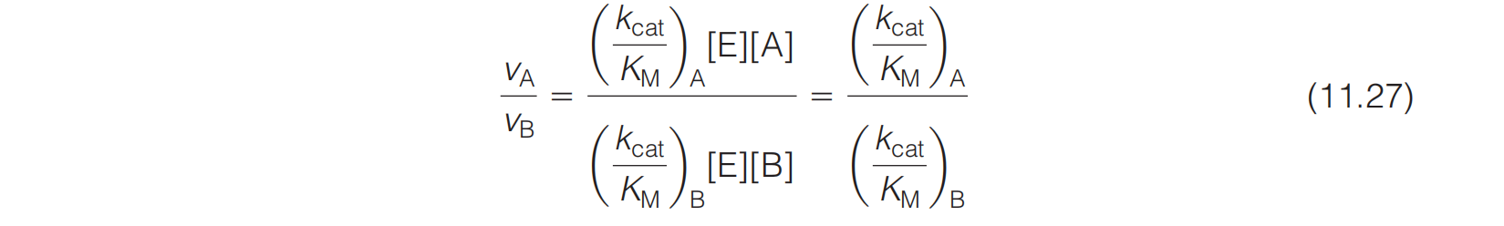
We have just seen that the ratio $k_{cat}/K_{M}$ corresponds to the second-order rate constant for enzyme–substrate combination under circumstances of low substrate concentration.
二、Analysis of Kinetic Data: Testing the Michaelis–Menten Equation
The measurement of reaction velocity as a function of substrate concentration is used to determine whether an enzyme-catalyzed reaction follows the Michaelis–Menten model (equation 11.25)
$$
v = \frac{V_{max} [S]}{K_{M} + [S]}
$$
and, if so, to determine the constants $K_{M} \text{ and } k_{cat}$
Analysis of initial rates
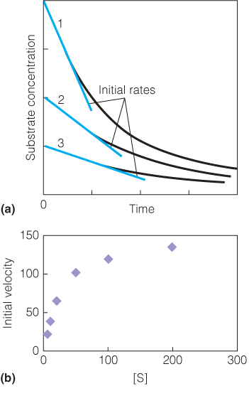
Several reactions are performed with varying concentrations of substrate and the values of the initial rates are determined from the slopes of the curves in the early phase for each reaction.
Initial rate data, determined as described in panel A, are plotted as a function of the substrate concentration.
The enzyme appears to obey the Michaelis–Menten kinetic model.
Lineweaver–Burk plot 莱恩威弗-伯克作图
1. Deduction
Lineweaver–Burk plot is also called double reciprocal plot (双倒数图)
A Lineweaver–Burk plot provides a quick test for adherence to Michaelis–Menten kinetics and allows easy evaluation of the critical constants.
$$
\because v = \frac{V_{max} [S]}{K_{M} + [S]}
$$
$$
\text{两边取倒数得:}\frac{1}{v} = \frac{K_{M} + [S]}{V_{max} [S]}
$$
$$
\therefore \frac{K_{M} + [S]}{V_{max} [S]} = \frac{K_{M}}{V_{max} [S]} + \frac{1}{V_{max}}
$$
$$
\therefore \frac{1}{v} = (\frac{K_{M}}{V_{max}}) \frac{1}{[S]} + \frac{1}{V_{max}}
$$
Figure 11.25:

At 1/[S] = 0, [S] is infinitely large and the reaction velocity is at its maximum.

where denotes the value of $[S]_{0}$ at We then obtain from Equation 11.29:

2. Disadvantages
A disadvantage of a Lineweaver–Burk plot is that a long extrapolation(外推) is often required to determine $K_{M} $, which introduces corresponding uncertainty in the result.
Eadie–Hofstee plot
1. Deduction
$$
\text{Get from equation 11.25: }v = \frac{V_{max} [S]}{K_{M} + [S]}
$$
$$
\text{将右端算式的分母左乘:} v K_{M} + v [S] = V_{max} [S]
$$
$$
\text{左右同除[S]: } \frac{v K_{M}}{[S]} + v = V_{max}
$$
$$
\therefore v = V_{max} - \frac{v K_{M}}{[S]}
$$
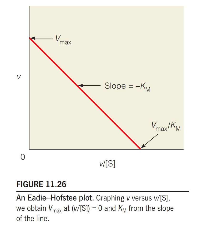
These linear plots provide useful methods for recognizing modes of inhibition; however, they suffer from unequal weighting of the data.
Performing nonlinear curve fitting to the raw data with readily available software is now preferred.
The observed effects of an amino acid mutation in an enzyme active site on $K_{M}$ and $k_{cat}$ can be used to identify the role of the amino acid in substrate binding ($K_{M}$ effects) and transition-state stabilization ($k_{cat}$ effects).
三、Multisubstrate Reactions
An example we have already discussed is proteolysis, which involves two substrates (the polypeptide and water) and two products (the two fragments of the cleaved polypeptide chain). Phosphorylation of glucose, as catalyzed by hexokinase, is another such case: The two substrates are glucose and ATP, and the products are glucose-6-phosphate and ADP.
When an enzyme binds two or more substrates and releases multiple products, the order of the steps becomes an important feature of the enzyme mechanism.
We shall illustrate them with examples using two substrates, S1 and S2, and two products, P1 and P2.
Random Substrate Binding
In random substrate binding, either substrate can be bound first, although in many cases one substrate will be favored for initial binding, and its binding may promote the binding of the other.
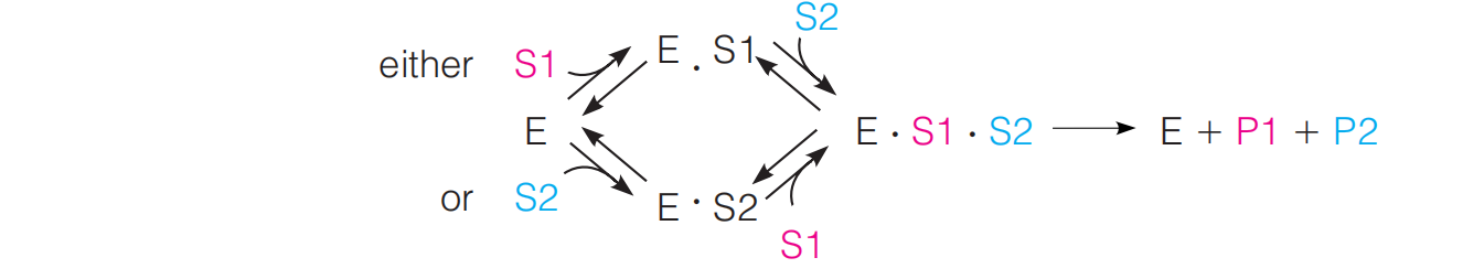
Example:
The phosphorylation of glucose by ATP, with hexokinase as the enzyme, appears to follow such a mechanism, although there is some tendency for glucose to bind first.
Ordered Substrate Binding
In some cases, one substrate must bind before a second substrate can bind significantly:

Example:
This mechanism is often observed in oxidations of substrates by the cofactor $NAD^{+}$ which is related to the cofactor $NADP^{+}$ discussed above in the dihydrofolate reductase mechanism.
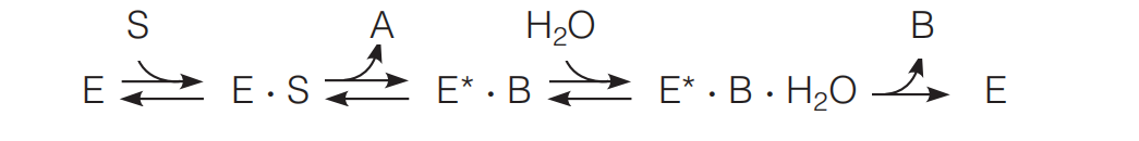
The Ping-Pong Mechanism
Sometimes the sequence of events in catalysis goes like this: One substrate is bound, one product is released, a second substrate comes in, and a second product is released. This is called a “ping-pong” reaction:
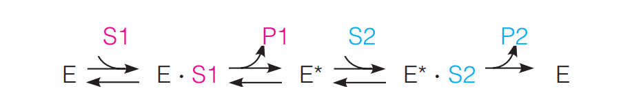
Here E* is a modified form of the enzyme, often carrying a fragment of S1.
A good example is the cleavage of a polypeptide chain by a serine protease such as trypsin or chymotrypsin.