02. R <- 基本绘图Ⅰ
这篇文章摘录了绘制一些基本图表的方法
一、条形图 (Bar Chart)
在条形图的例子当中使用了随vcd包分发的Arthritis数据框:library(vcd),可以通过vcd来创建棘状图(spinogram)。
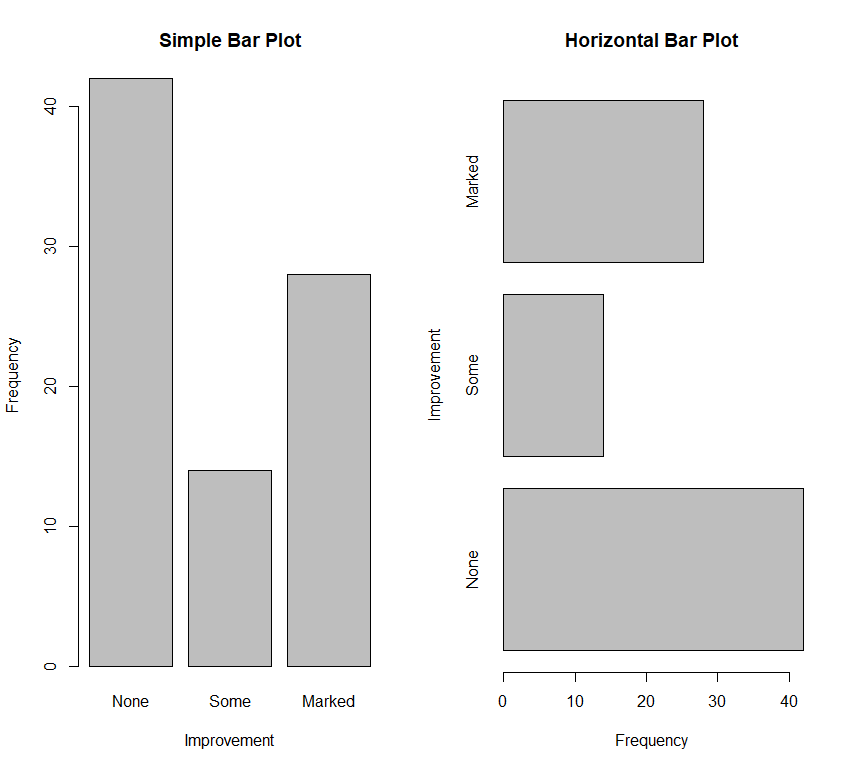
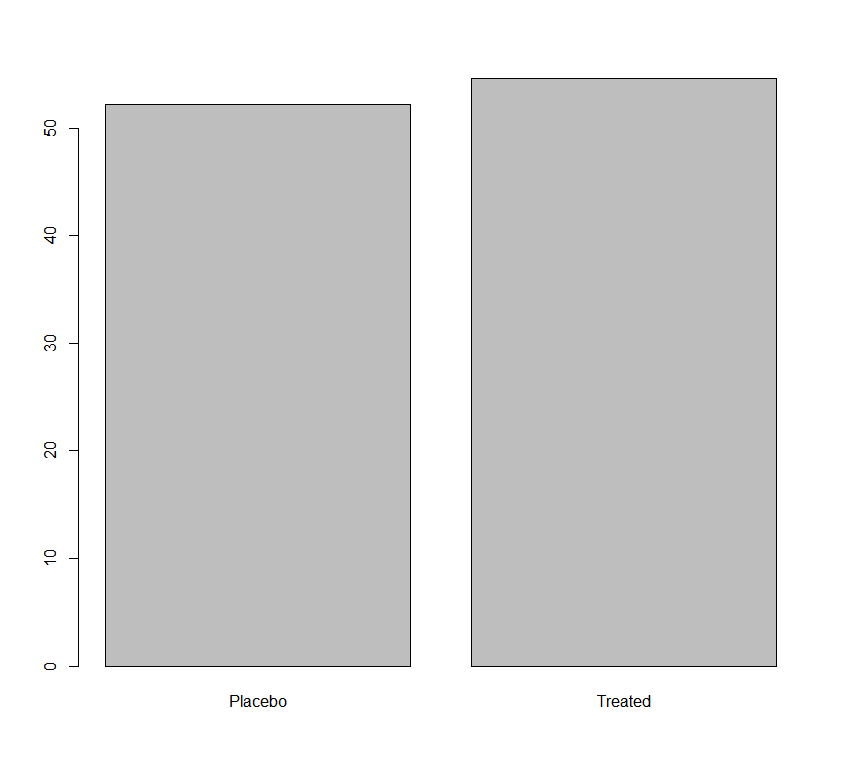
基本条形图
使用函数barplot()来创建基本条形图,大多数主要参数与其它图像是通用的,其中需要注意的主要参数有:
| 参数 | 描述 |
|---|---|
| height | height是一个向量或一个矩阵,它是绘图过程中每个bar的值(高度) |
| horiz | 默认为FALSE,若horiz=TRUE则会生成水平条形图 |
例:
本例中使用的数据:
1 | |
绘图代码:
1 | |
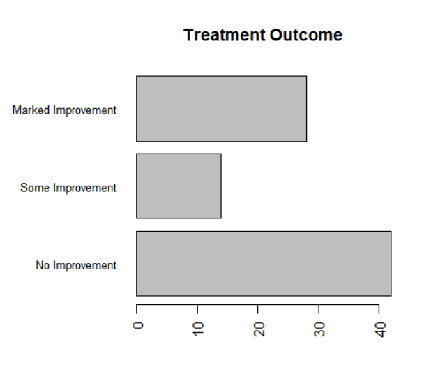
1. 条形图的微调
可以使用参数cex.names来减小字号。将其指定为小于1的值可以缩小标签的大小。可选的参数names.arg允许你指定一个字符向量作为条形的标签名。你同样可以使用图形参数辅助调整文本间隔。
| 参数 | 描述 |
|---|---|
| las | numeric in {0,1,2,3}; the style of axis labels. 0: always parallel to the axis [default], 1: always horizontal, 2: always perpendicular to the axis, 3: always vertical. Also supported by mtext. Note that string/character rotation via argument srt to par does not affect the axis labels. |
例:
1 | |
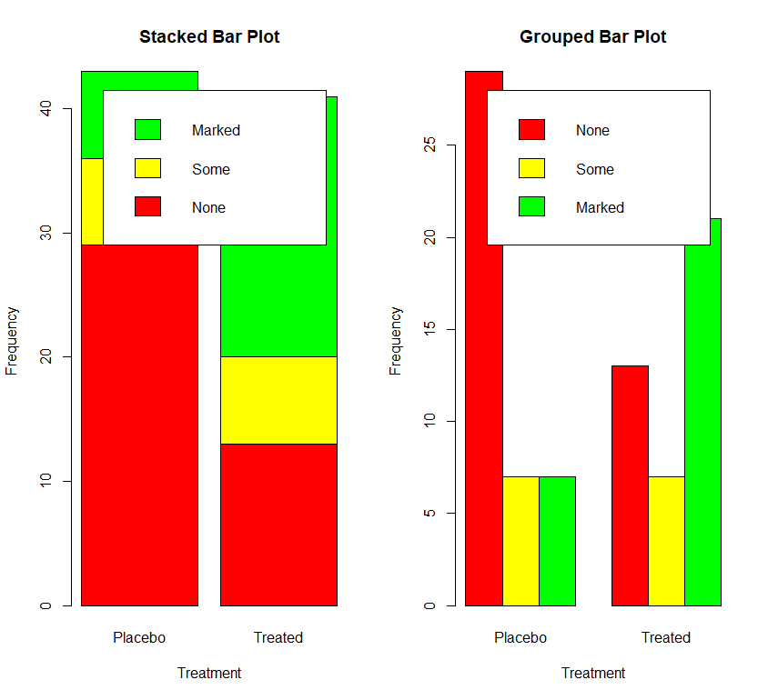
堆砌条形图与分组条形图
如果height是一个矩阵而不是一个向量,则绘图结果将是一幅堆砌条形图或分组条形图。
堆砌条形图与分组条形图中的重要参数为:
| 参数 | 描述 |
|---|---|
| beside | 若beside=FALSE(默认值),则矩阵中的每一列都将生成图中的一个条形,各列中的值将给出 堆砌的“子条”的高度。 若beside=TRUE,则矩阵中的每一列都表示一个分组,各列中的值将并列而不是堆砌。 |
例:
本例中使用的数据:
1 | |
绘图代码:
1 | |
均值条形图
条形图并不一定要基于计数数据或频率数据。可以使用数据整合函数并将结果传递给barplot()函数,来创建表示均值、中位数、标准差等的条形图。
本例中使用的数据:
1 | |
绘图代码:
1 | |
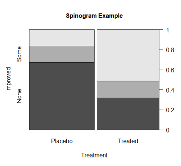
棘状图
棘状图对堆砌条形图进行了重缩放,这样每个条形的高度均为1,每一段的高度即表示比例。棘状图可由vcd包中的函数spine()绘制。
例:
使用的数据:
1 | |
绘图代码:
1 | |
二、饼图 (Pie Chart)
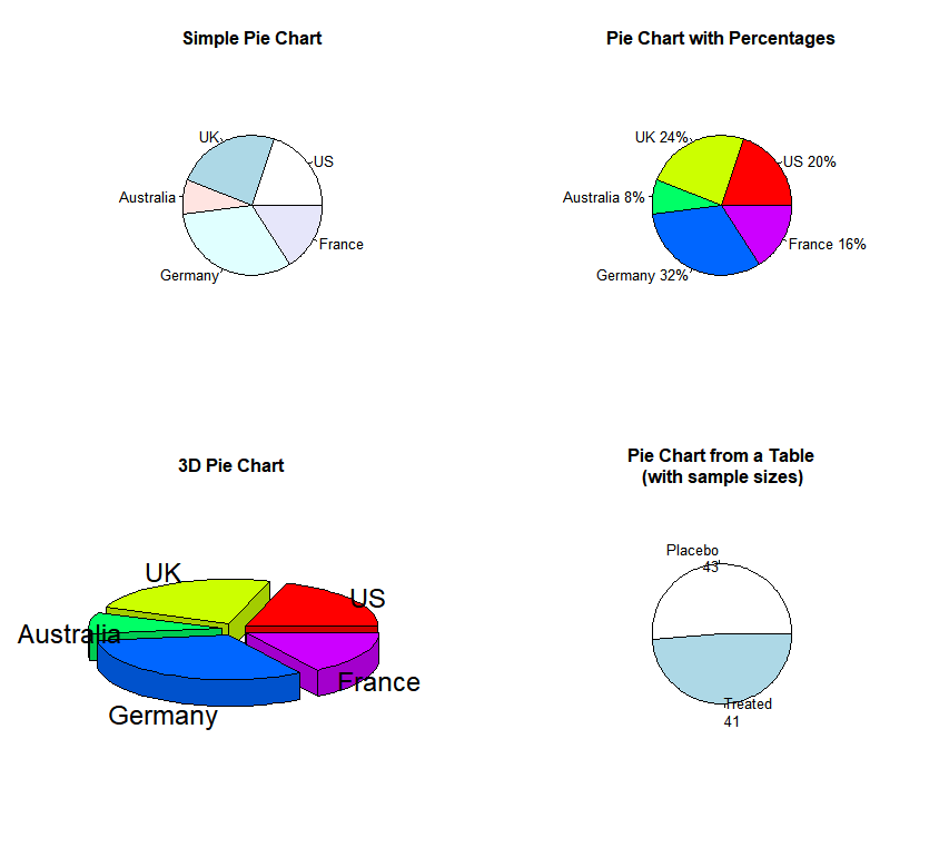
经典饼图
饼图的绘图函数是 pie(x, labels),当绘制3D饼图的时候,需要使用 plotrix 包中的 pie3D() 函数
| 参数 | 描述 |
|---|---|
| x | 一个非负数值向量,表示每个扇形的面积 |
| labels | 表示各扇形标签的字符型向量。 |
例:
使用的数据:
1 | |
绘图参数:
1 | |
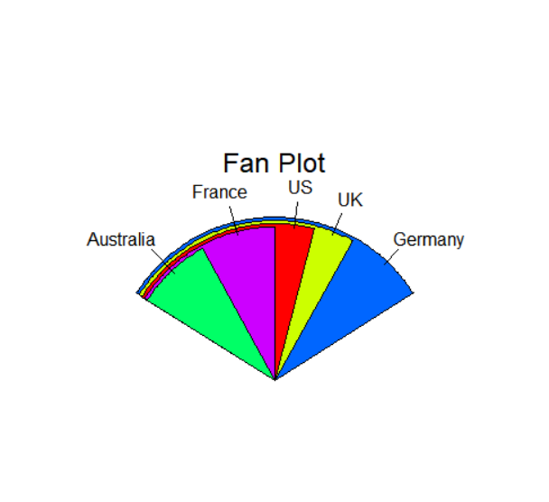
扇形图
扇形图(fan plot)是饼图的变种。扇形图提供了一种同时展示相对数量和相互差异的方法。在R中,扇形图是通过plotrix包中的fan.plot()函数实现的。
例:
1 | |
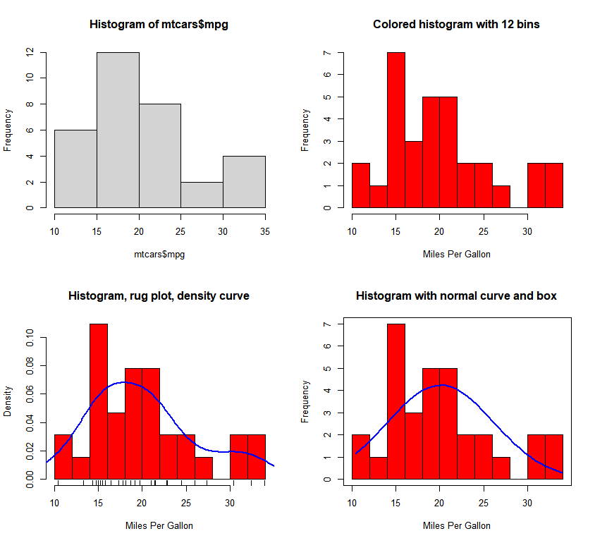
三、直方图 (Histogram)
直方图通过在x轴上将值域分割为一定数量的组,在y轴上显示相应值的频数,展示了连续型变量的分布。可以使用如下函数创建直方图:hist(x)
| 参数 | 描述 |
|---|---|
| x | 一个由数据值组成的数值向量 |
| freq | freq=FALSE表示根据概率密度而不是频数绘制图形 |
| breaks | 控制组的数量。在定义直方图中的单元时,默认将生成等距切分。 |
部分常用函数解释
1. 轴须图相关
函数 jitter: ‘Jitter’ (Add Noise) to Numbers
- Add a small amount of noise to a numeric vector.
- Usage:
jitter(x, factor = 1, amount = NULL)
| 参数 | 描述 |
|---|---|
| x | numeric vector to which jitter should be added. |
| factor | numeric value. |
| amount | numeric; if positive, used as amount (see below), otherwise, if = 0 the default is factor * z/50. Default (NULL): factor * d/5 where d is about the smallest difference between x values. |
函数 rug: Add a Rug to a Plot
- Adds a rug representation (1-d plot) of the data to the plot.
- Usage:
rug(x, ticksize = 0.03, side = 1, lwd = 0.5, col = par("fg"), quiet = getOption("warn") < 0, ...)
| 参数 | 描述 |
|---|---|
| x | A numeric vector |
| ticksize | The length of the ticks making up the ‘rug’. Positive lengths give inwards ticks. |
| side | On which side of the plot box the rug will be plotted. Normally 1 (bottom) or 3 (top). |
| lwd | The line width of the ticks. Some devices will round the default width up to 1. |
| col | The colour the ticks are plotted in. |
| quiet | logical indicating if there should be a warning about clipped values. |
| … | further arguments, passed to axis, such as line or pos for specifying the location of the rug. |
函数 lines: Add Connected Line Segments to a Plot
- A generic function taking coordinates given in various ways and joining the corresponding points with line segments.
lines(x,y)是在给定x, y两个向量之后,将x,y中的每一个元素对应为一些点,然后把这些点用平滑的曲线连接。
- Usage:
lines(x, ...)
| 参数 | 描述 |
|---|---|
| x, y | coordinate vectors of points to join. |
| … | Arguments the same as par |
2. 正态曲线相关
函数 dnorm, pnorm, qnorm, rnorm: The Normal Distribution
- Density, distribution function, quantile function and random generation for the normal distribution with mean equal to mean and standard deviation equal to sd.
- Usage:
dnorm(x, mean = 0, sd = 1, log = FALSE)pnorm(q, mean = 0, sd = 1, lower.tail = TRUE, log.p = FALSE)qnorm(p, mean = 0, sd = 1, lower.tail = TRUE, log.p = FALSE)rnorm(n, mean = 0, sd = 1)
| 参数 | 描述 |
|---|---|
| x, q | vector of quantiles. |
| p | vector of probabilities. |
| n | number of observations. If length(n) > 1, the length is taken to be the number required. |
| mean | vector of means. |
| sd | vector of standard deviations. |
| log, log.p | logical; if TRUE, probabilities p are given as log(p). |
| lower.tail | logical; if TRUE (default), probabilities are P[X ≤ x] otherwise, P[X > x]. |
3. 直方图 + (轴须图,正态密度曲线)
例:
1 | |
四、核密度图
这部分不涉及使用 ggplot2 的情况
绘制核密度图
核密度曲线类似于概率密度曲线,其曲线下的面积是1,因此其y轴上的单位通常是小于1的核密度分布值。对这个核密度曲线求积分的结果为1,也就是其曲线下的面积为1。
绘制密度图的方法(不叠加到另一幅图上方)为:plot(density(x))
- 其中的
x是一个数值型向量。由于plot()函数会创建一幅新的图形,所以要向一幅已经存在的图形上叠加一条密度曲线,可以使用lines()函数
例:
1 | |
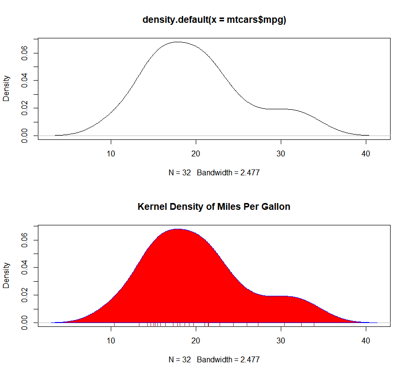
polygon()函数根据顶点的x和y坐标(本例中由density()函数提供)绘制了多边形。
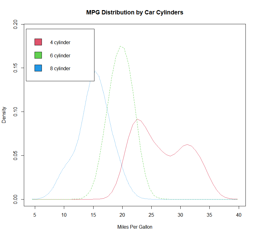
比较核密度图
这部分使用到了包 sm
核密度图可用于比较组间差异。可能是由于普遍缺乏方便好用的软件,这种方法其实完全没有被充分利用。幸运的是,sm包漂亮地填补了这一缺口。
使用sm包中的sm.density.compare()函数可向图形叠加两组或更多的核密度图。使用格式为:
sm.density.compare(x, factor)
| 参数 | 描述 |
|---|---|
| x | 一个数值型向量 |
| factor | 是一个分组变量 |
例:
1 | |
- 对图例部分的说明:首先创建的是一个颜色向量,这里的
colfill值为c(2, 3, 4)。然后通过legend()函数向图形上添加一个图例。第一个参数值locator(1)表示用鼠标点击想让图例出现的位置来交互式地放置这个图例。第二个参数值则是由标签组成的字符向量。第三个参数值使用向量colfill为cyl.f的每一个水平指定了一种颜色。
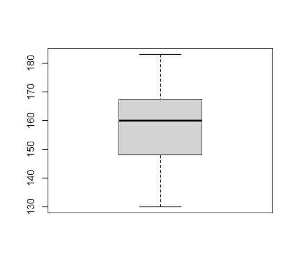
五、箱线图 (Box Plot)
箱线图的标注
箱线图(又称盒须图)通过绘制连续型变量的五数总括,即最小值、下四分位数(第25百分位数)、中位数(第50百分位数)、上四分位数(第75百分位数)以及最大值,描述了连续型变量的分布。箱线图能够显示出可能为离群点(范围 ±1.5*IQR 以外的值,IQR表示四分位距,即上四分位数与下四分位数的差值)的观测。例如:boxplot(mtcars$mpg, main="Box plot", ylab="Miles per Gallon")

- 默认情况下,两条须的延伸极限不会超过盒型各端加1.5倍四分位距的范围。此范围以外的值将以点 (outlier) 来表示
绘制箱线图
箱线图可以展示单个变量或分组变量。使用格式为
boxplot(formula, data=dataframe)
| 参数 | 描述 |
|---|---|
| x | 向量,列表或数据框。 |
| formula | 公式,形如y~grp,其中y为向量,grp是数据的分组,通常为因子。 具体的介绍看此表之后 |
| range | 数值,默认为1.5,表示触须的范围,即range × (Q3 - Q1) |
| width | 箱体的相对宽度,当有多个箱体时,有效。 |
| data | 提供数据的数据框(或列表), 用于提供公式中的数据。 |
| varwidth | 逻辑值,控制箱体的宽度, 只有图中有多个箱体时才发挥作用,默认为FALSE, 所有箱体的宽度相同,当其值为TRUE时,代表每个箱体的样本量作为其相对宽度 varwidth=TRUE将使箱线图的宽度与其样本大小的平方根成正比 |
| notch | 逻辑值,如果该参数设置为TRUE,则在箱体两侧会出现凹口。默认为FALSE。 |
| outline | 逻辑值,如果该参数设置为FALSE,则箱线图中不会绘制离群值。默认为TRUE |
| names | 绘制在每个箱线图下方的分组标签 |
| plot | 逻辑值,是否绘制箱线图,如设置为FALSE,则不绘制箱线图,而给出绘制箱线图的相关信息,如5个点的信息等。 |
| border | 箱线图的边框颜色 |
| col | 箱线图的填充色。 |
| horizontal | 逻辑值,指定箱线图是否水平绘制,默认为FALSE。 horizontal=TRUE可以反转坐标轴的方向 |
对于 formula 的解释:
y ~ A,这将为类别型变量A的每个值并列地生成数值型变量y的箱线图- 公式
y ~ A*B则将为类别型变量A和B所有水平的两两组合生成数值型变量y的箱线图
例:
1 | |
1. 单组箱线图
直接使用 boxplot(x) 实现:
1 | |
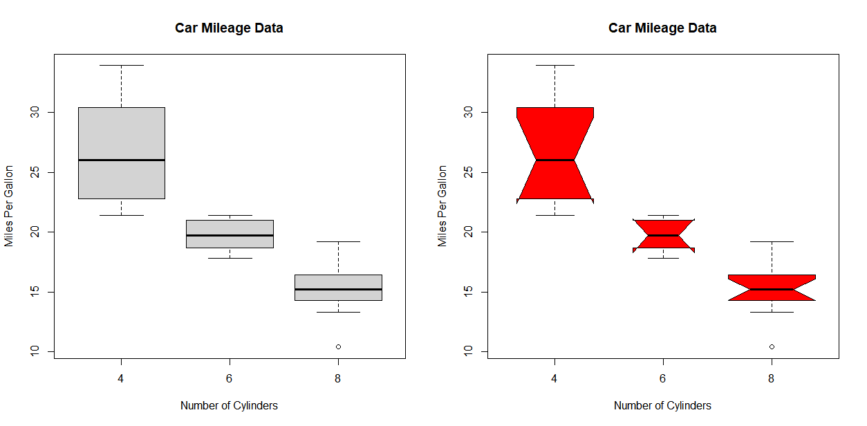
2. 多组箱线图
单交叉因子和凹槽
需要设置 boxplot 中的 formula, data 等参数:
当 notch = TRUE 的时候,箱线图含凹槽
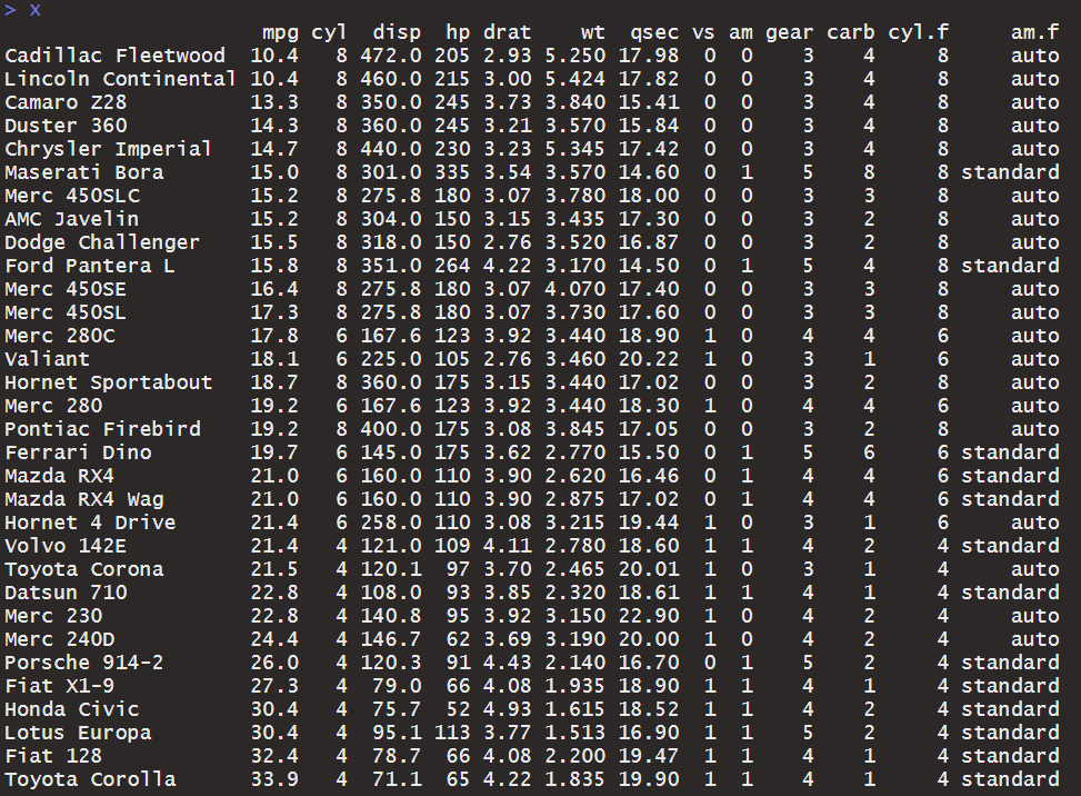
绘图代码:使用了预设数据集 mtcars 中的 mpg , cyl
1 | |
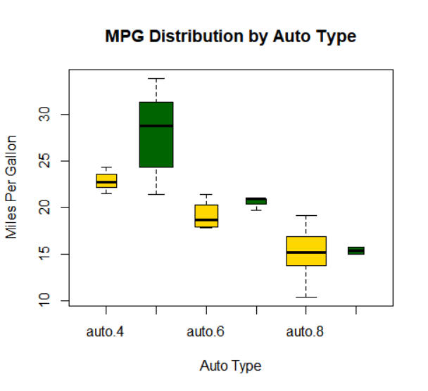
多交叉因子
绘图代码:使用了预设数据集 mtcars 中的 mpg , cyl 和 am
1 | |
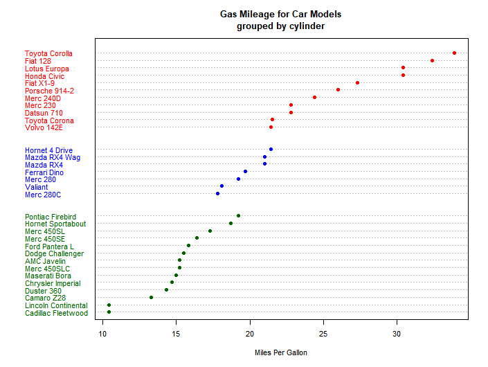
六、点图 (Point Plot, Dot Chart)
绘制经典点图
点图提供了一种在简单水平刻度上绘制大量有标签值的方法。你可以使用dotchart()函数创建点图,格式为:dotchart(x, labels=)
| 参数 | 描述 |
|---|---|
| x | 是一个数值向量 |
| labels | 由每个点的标签组成的向量 |
| groups | 可以通过添加参数groups来选定一个因子,用以指定x中元素的分组方式。如果这样做,则参数gcolor可以控制不同组标签的颜色,cex可以控制标签的大小。 |
例:
1 | |

分组、排序、着色后的点图
例:
涉及的数据:
1 | |
1 | |