05. R <- 独立性、相关性、假设检验以及相关统计量

一、Sampling Distribution (抽样分布)

相关概念

1. Point Estimation

Population	Sample
Population mean: $E[X] = \mu$	Sample mean: $\bar{x} = \frac{1}{n} \sum^{n}{i=1} x{x}$
Population variance: $var(X) = \sigma^{2}$	Sample variance: $s^{2} = \frac{1}{n-1} \sum^{n}{i=1} (x{i} - \bar{x})^{2}$
Population standard deviation: $\sigma_{X} = \sqrt{var(X)} = \sigma$	Sample standard deviation: s = $\sqrt{\frac{\sum^{n}{i=1}{(x{i}-\bar{x})^{2}}}{n-1}}$
Parameters	Descriptive Statistics

	Population distribution	Sample distribution	Sampling distribution of the sample mean
Mean	$\mu$	$\bar{x}$	$\mu_{\bar{X}}$
Variance	$\sigma^{2}$	$s^{2}$	$\sigma_{\bar{X}}^{2}$
Standard deviation	$\sigma$	$s$	$\sigma_{\bar{X}}$

2. In Hypothesis Test

Term	Description
$Z$, $t$, $\Chi$; …	Test statistic.
$p$	p-value
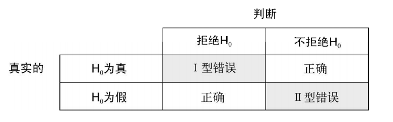
$\alpha$	Significant Level; The probability of making a type I error $\alpha$ = P(reject H0 | H0 is true).
$\beta$	The probability of committing a type II error $\beta$ = P(do not reject H0 | H0 is false).
$1-\beta$	Power; power = P(reject H0 | H0 is false)

3. Interval Estimation - Confidence Interval 置信区间

Confidence Interval for The Mean

若总体方差 (Population Variance, $\sigma^{2}$)已知，可以直接使用它来计算出样本的置信区间，涉及正态分布

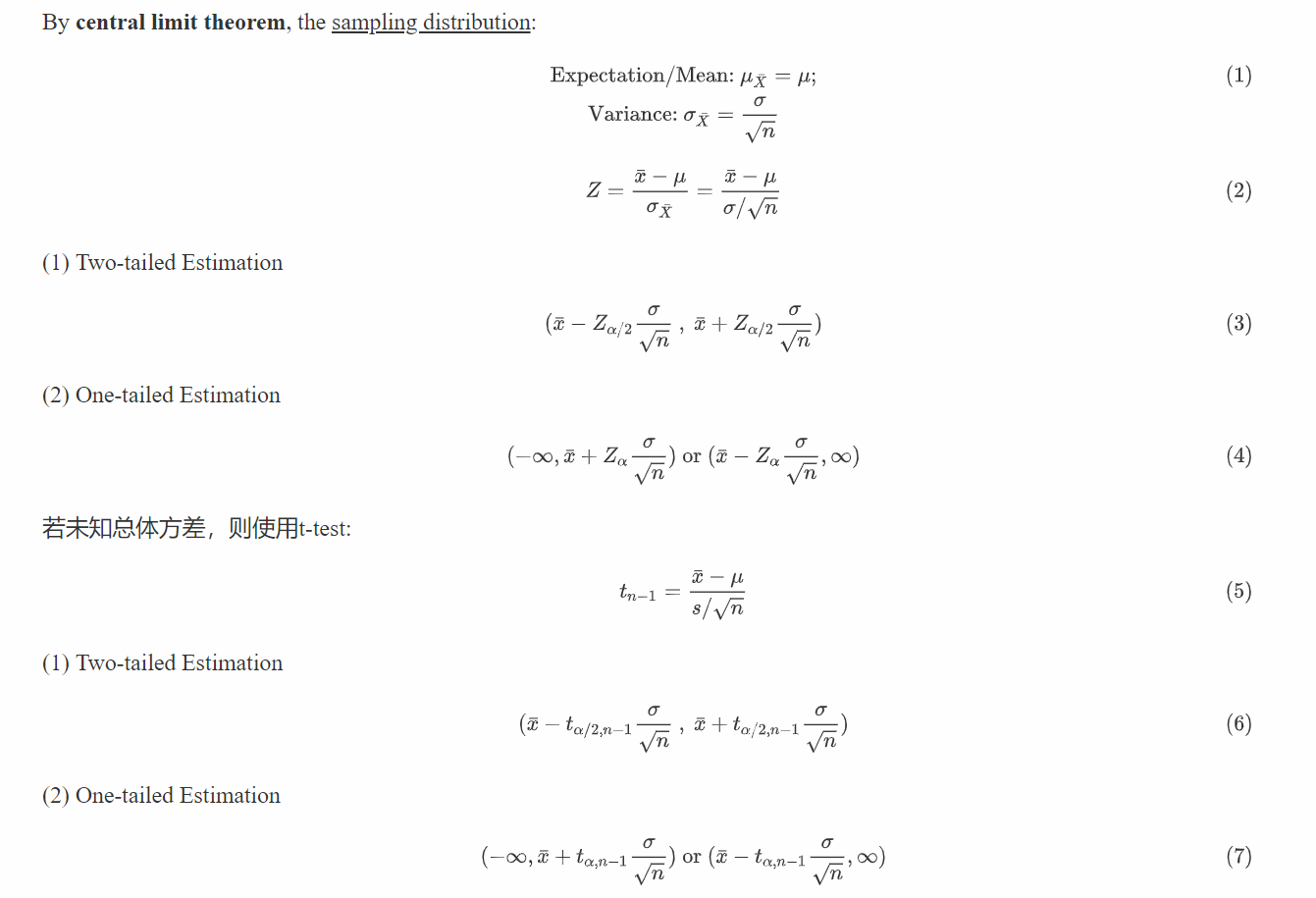
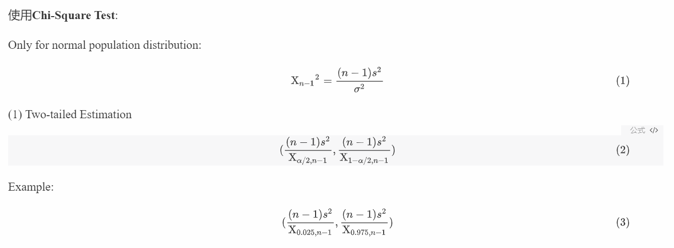
Confidence Interval for The Variance

只有在样本正态分布的时候，才可以使用此方法估计方差的样本空间。

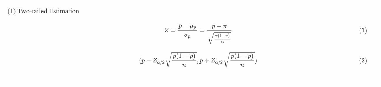
Interval for proportion

涉及比例的时候，使用正态分布相关对置信区间进行估计：

4. 连续性矫正 (Continuity Correction)

当满足n足够大，p不过小，np>5或者nq<30的条件时，可近似地采用u检验法，就是有连续性矫正，即正态近似法来进行显著性检验；

在R中的检验函数中通过参数correct进行设置。

二、假设检验 (Hypothesis Test)

相关概念

在统计假设检验中，首先要对总体分布参数设定一个假设（零假设，H0），然后从总体分布中抽样，通过样本计算所得的统计量来对总体参数进行推断。假定零假设为真，如果计算获得观测样本的统计量的概率非常小，便可以拒绝原假设，接受它的对立面（称作备择假设或者研究假设，H1）。

在假设检验当中，通常会提到两种错误：

相关函数

1. Testing for Means: t-test

在这一部分当中，使用MASS包的UScrime数据集来进行示范：

> library(MASS)
> head(UScrime)
    M So  Ed Po1 Po2  LF  M.F Pop  NW  U1 U2 GDP Ineq     Prob    Time    y
1 151  1  91  58  56 510  950  33 301 108 41 394  261 0.084602 26.2011  791
2 143  0 113 103  95 583 1012  13 102  96 36 557  194 0.029599 25.2999 1635
3 142  1  89  45  44 533  969  18 219  94 33 318  250 0.083401 24.3006  578
4 136  0 121 149 141 577  994 157  80 102 39 673  167 0.015801 29.9012 1969
5 141  0 121 109 101 591  985  18  30  91 20 578  174 0.041399 21.2998 1234
6 121  0 110 118 115 547  964  25  44  84 29 689  126 0.034201 20.9995  682

t检验涉及到t分布（t distribution）:

独立样本的 t 检验

假设两组数据是独立的，并且是从正态总体中抽得。一种检验的调用格式为：

t.test(y ~ x, data)

• y是一个数值型变量，x是一个二分变量

另外一种调用格式为：

t.test(y1, y2)

• 其中的y1和y2为数值型向量（即各组的结果变量）。
• 可选参数data的取值为一个包含了这些变量的矩阵或数据框。

即：

Default S3 method:
t.test(x, y = NULL, alternative = c("two.sided", "less", "greater"), mu = 0, paired = FALSE, var.equal = FALSE, conf.level = 0.95, ...)

S3 method for class ‘formula’:

t.test(formula, data, subset, na.action, ...)

注：

1. 这里的t检验默认假定方差不相等，并使用Welsh的修正自由度。你可以添加一个参数var.equal=TRUE以假定方差相等，并使用合并方差估计。
2. 默认的备择假设是双侧的（即均值不相等，但大小的方向不确定）。你可以添加一个参数alternative="less"或alternative="greater"来进行有方向的检验。

参数表:

参数	描述
y1 (x), y2 (y)	数值型向量，也可以是matrix。 当x为matrix时，y会被忽略
var.equal=	var.equal=TRUE以假定方差相等，并使用合并方差估计。 默认为FLASE
alternative=	设置该参数为：alternative="less"或alternative="greater"来进行有方向的检验 默认为双侧检验
conf.level=	confidence level of the interval
mu	a number indicating the true value of the mean (or difference in means if you are performing a two sample test).

例：

# 简化后续代码
> library(MASS)
> attach(UScrime)

# Welch Two Sample t-test
> t.test(Prob, GDP)

	Welch Two Sample t-test

data:  Prob and GDP
t = -37.325, df = 46, p-value < 2.2e-16
alternative hypothesis: true difference in means is not equal to 0
95 percent confidence interval:
 -553.6667 -497.0051
sample estimates:
   mean of x    mean of y 
  0.04709138 525.38297872 

# 当两个数据组的方差相等时，不使用Welch Method调整方差
> t.test(Prob, GDP, var.equal = TRUE)

	Two Sample t-test

data:  Prob and GDP
t = -37.325, df = 92, p-value < 2.2e-16
alternative hypothesis: true difference in means is not equal to 0
95 percent confidence interval:
 -553.2894 -497.3824
sample estimates:
   mean of x    mean of y 
  0.04709138 525.38297872 

# One-sided t test，此时置信区间在右侧
> t.test(Prob, GDP, alternative = "less")

	Welch Two Sample t-test

data:  Prob and GDP
t = -37.325, df = 46, p-value < 2.2e-16
alternative hypothesis: true difference in means is less than 0
95 percent confidence interval:
      -Inf -501.7093
sample estimates:
   mean of x    mean of y 
  0.04709138 525.38297872 

# One-sided t test，此时置信区间在左侧
> t.test(Prob, GDP, alternative = "greater")

	Welch Two Sample t-test

data:  Prob and GDP
t = -37.325, df = 46, p-value = 1
alternative hypothesis: true difference in means is greater than 0
95 percent confidence interval:
 -548.9624       Inf
sample estimates:
   mean of x    mean of y 
  0.04709138 525.38297872 

# 指定求50%的置信区间
> t.test(Prob, GDP, conf.level = .5)

	Welch Two Sample t-test

data:  Prob and GDP
t = -37.325, df = 46, p-value < 2.2e-16
alternative hypothesis: true difference in means is not equal to 0
50 percent confidence interval:
 -534.9047 -515.7671
sample estimates:
   mean of x    mean of y 
  0.04709138 525.38297872 

> detach(UScrime)

非独立样本的 t 检验

非独立样本的t检验假定组间的差异呈正态分布。对于本例，检验的调用格式为：

t.test(y1, y2, paired = TRUE)

例：针对UScrime数据集当中的两个数据组U1和U2进行分析

> library(MASS)
> attach(UScrime)

# 对这两个数据集进行初步分析
> sapply(UScrime[c("U1","U2")], function(x)(c(mean=mean(x),sd=sd(x))))
           U1       U2
mean 95.46809 33.97872
sd   18.02878  8.44545
         
# Paired t test
> t.test(U1, U2, paired = TRUE)

	Paired t-test

data:  U1 and U2
t = 32.407, df = 46, p-value < 2.2e-16
alternative hypothesis: true difference in means is not equal to 0
95 percent confidence interval:
 57.67003 65.30870
sample estimates:
mean of the differences 
               61.48936 

> detach(UScrime)

2. Testing for Variances: Chi-Square and F Test

One-sample hypothesis testing for variance： Chi-Square Test

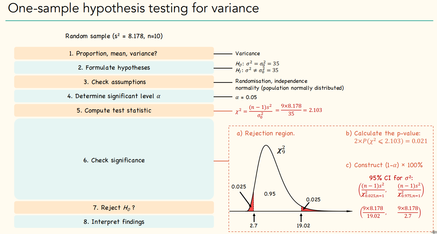
对于单样本的假设检验，需要使用到卡方检验 (Chi-Square test)，使用格式如下：

chisq.test(x, y = NULL, correct = TRUE, p = rep(1/length(x), length(x)), rescale.p = FALSE, simulate.p.value = FALSE, B = 2000)

参数	描述
x, y	数值型向量，也可以是matrix。 当x为matrix时，y会被忽略
correct	该逻辑参数控制2x2列联表的独立性检验时，是否进行连续性矫正，即对所有$
p	输入的概率值，应与x变量的长度一致。注意p不可以为负数
rescale.p	该逻辑参数控制是否将p的和重新调整为1
simulate.p.value	控制是否以蒙特卡洛采样的方法模拟p值
B	蒙特卡洛采样的重复次数

例，使用MASS包的UScrime数据集来进行示范比较U1和U2：

> library(MASS)
> head(Uscrime)
    M So  Ed Po1 Po2  LF  M.F Pop  NW  U1 U2 GDP Ineq     Prob    Time    y
1 151  1  91  58  56 510  950  33 301 108 41 394  261 0.084602 26.2011  791
2 143  0 113 103  95 583 1012  13 102  96 36 557  194 0.029599 25.2999 1635
3 142  1  89  45  44 533  969  18 219  94 33 318  250 0.083401 24.3006  578
4 136  0 121 149 141 577  994 157  80 102 39 673  167 0.015801 29.9012 1969
5 141  0 121 109 101 591  985  18  30  91 20 578  174 0.041399 21.2998 1234
6 121  0 110 118 115 547  964  25  44  84 29 689  126 0.034201 20.9995  682

> chisq.test(U1, U2)

	Pearson's Chi-squared test

data:  U1 and U2
X-squared = 877.07, df = 850, p-value = 0.2527

Warning message:
In chisq.test(U1, U2) : Chi-squared近似算法有可能不准

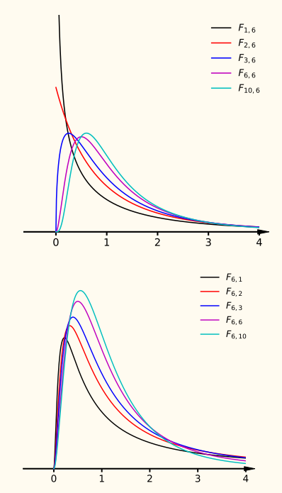
Testing for The Equality of Two variances: F-test

相关概念

Uses the F distribution（统计值服从F-分布的检验）

Let:
$$
U_{1} = \frac{(n_{1}-1)s_{1}^{2}}{\sigma_{1}^2}, U_{2} = \frac{(n_{2}-1)s_{2}^{2}}{\sigma_{2}^2}
$$
The test statistic:
$$
F = \frac{U_{1}/v_{1}}{U_{2}/v_{2}} = \frac{\frac{(n_{1}-1)s_{1}^{2}}{\sigma_{1}^2}/(n_{1}-1)}{\frac{(n_{2}-1)s_{2}^{2}}{\sigma_{2}^2}/(n_{2}-1)} =
\frac{s_{1}^{2}}{s_{2}^{2}} \cdot \frac{\sigma_{2}^{2}}{\sigma_{1}^{2}}
$$

相关函数

在R中，使用F test的时候，可以通过函数var.test()来实现，和t.test()相似，它也有两种使用格式：

Default S3 method:
var.test(x, y, ratio = 1, alternative = c("two.sided", "less", "greater"), conf.level = 0.95, ...)

S3 method for class ‘formula’:

var.test(formula, data, subset, na.action, ...)

参数	描述
x, y	数值型向量，也可以是matrix。 当x为matrix时，y会被忽略
ratio	the hypothesized ratio of the population variances of x and y.

例，使用MASS包的UScrime数据集来进行示范比较U1和U2：

> library(MASS)
> head(UScrime)
    M So  Ed Po1 Po2  LF  M.F Pop  NW  U1 U2 GDP Ineq     Prob    Time    y
1 151  1  91  58  56 510  950  33 301 108 41 394  261 0.084602 26.2011  791
2 143  0 113 103  95 583 1012  13 102  96 36 557  194 0.029599 25.2999 1635
3 142  1  89  45  44 533  969  18 219  94 33 318  250 0.083401 24.3006  578
4 136  0 121 149 141 577  994 157  80 102 39 673  167 0.015801 29.9012 1969
5 141  0 121 109 101 591  985  18  30  91 20 578  174 0.041399 21.2998 1234
6 121  0 110 118 115 547  964  25  44  84 29 689  126 0.034201 20.9995  682

> attach(UScrime)
The following objects are masked from UScrime (pos = 3):

    Ed, GDP, Ineq, LF, M, M.F, NW, Po1, Po2, Pop, Prob, So, Time, U1, U2, y

> var.test(U1,U2)

	F test to compare two variances

data:  U1 and U2
F = 4.5571, num df = 46, denom df = 46, p-value = 9.637e-07
alternative hypothesis: true ratio of variances is not equal to 1
95 percent confidence interval:
 2.538310 8.181442
sample estimates:
ratio of variances 
          4.557086 

> detach(UScrime)

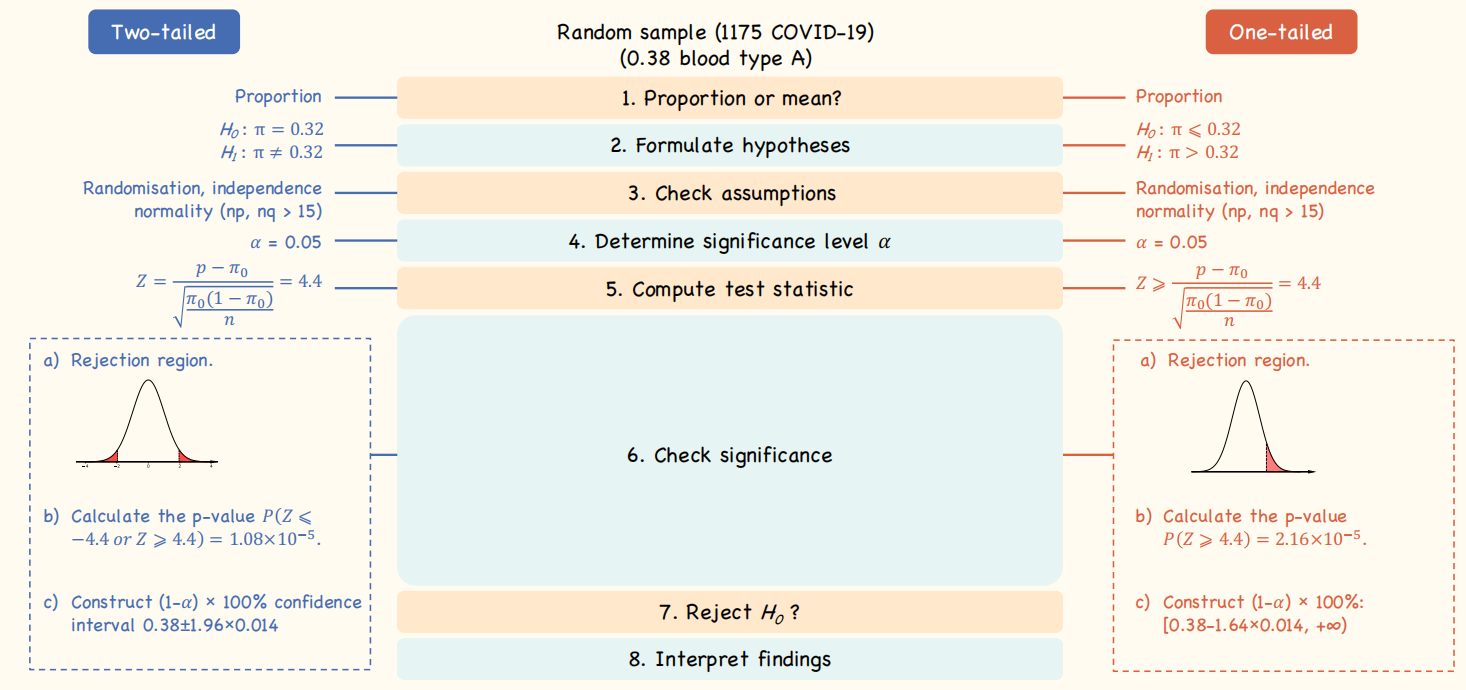
3. Testing for Proportions

One-sample hypothesis testing for proportion

当对样本的比例与总体进行假设检验的时候，需要使用z test，在R中可以通过函数prop.test实现：
prop.test(x, n, p = NULL, alternative = c("two.sided", "less", "greater"), conf.level = 0.95, correct = TRUE)

使用方法同之前的t.test()

例：1175个病人当中大约0.38的病人为A血型，检验此样本的A血型比例是否与之前得到的结论：”比例为0.32” 一致

> prop.test(446.5, 1175, p = 0.32, correct = FALSE)

	1-sample proportions test without continuity correction

data:  446.5 out of 1175, null probability 0.32
X-squared = 19.439, df = 1, p-value = 1.038e-05
alternative hypothesis: true p is not equal to 0.32
95 percent confidence interval:
 0.3526801 0.4081020
sample estimates:
   p 
0.38

> prop.test(446.5, 1175, p = 0.32, correct = FALSE, alternative = "less")

	1-sample proportions test without continuity correction

data:  446.5 out of 1175, null probability 0.32
X-squared = 19.439, df = 1, p-value = 1
alternative hypothesis: true p is less than 0.32
95 percent confidence interval:
 0.000000 0.403542
sample estimates:
   p 
0.38 

> prop.test(446.5, 1175, p = 0.32, correct = FALSE, alternative = "greater")

	1-sample proportions test without continuity correction

data:  446.5 out of 1175, null probability 0.32
X-squared = 19.439, df = 1, p-value = 5.192e-06
alternative hypothesis: true p is greater than 0.32
95 percent confidence interval:
 0.3570094 1.0000000
sample estimates:
   p 
0.38 

方差分析 (Analysis of Variance, ANOVA)

1. 相关概念

Source of Variance

方差分析的基本原理是认为不同处理组的均数间的差别基本来源有两个：

1. 实验条件，即不同的处理造成的差异，称为组间差异。用变量在各组的均值与总均值之偏差平方和的总和表示，记作$SS_{B}$，组间自由度$df_{B}$。
2. 随机误差，如测量误差造成的差异或个体间的差异，称为组内差异，用变量在各组的均值与该组内变量值之偏差平方和的总和表示， 记作$SS_{W}$，组内自由度$df_{W}$。

总偏差平方和 SST = SSB + SSW

基本思想

方差分析的基本思想是：通过分析研究不同来源的变异对总变异的贡献大小，从而确定可控因素对研究结果影响力的大小。

分析方法 根据资料设计类型的不同，有以下两种方差分析的方法：

1. 对成组设计的多个样本均值比较，应采用完全随机设计的方差分析，即单因素方差分析。
2. 对随机区组设计的多个样本均值比较，应采用配伍组设计的方差分析，即两因素方差分析。

单因素方差分析是用来研究一个控制变量的不同水平是否对观测变量产生了显著影响。这里，由于仅研究单个因素对观测变量的影响，因此称为单因素方差分析。

• 例如，分析不同施肥量是否给农作物产量带来显著影响，考察地区差异是否影响妇女的生育率，研究学历对工资收入的影响等。这些问题都可以通过单因素方差分析得到答案。

多因素方差分析用来研究两个及两个以上控制变量是否对观测变量产生显著影响。这里，由于研究多个因素对观测变量的影响，因此称为多因素方差分析。多因素方差分析不仅能够分析多个因素对观测变量的独立影响，更能够分析多个控制因素的交互作用能否对观测变量的分布产生显著影响，进而最终找到利于观测变量的最优组合。

• 例如：分析不同品种、不同施肥量对农作物产量的影响时，可将农作物产量作为观测变量，品种和施肥量作为控制变量。利用多因素方差分析方法，研究不同品种、不同施肥量是如何影响农作物产量的，并进一步研究哪种品种与哪种水平的施肥量是提高农作物产量的最优组合。
• 当设计包含两个甚至更多的因子时，便是因素方差分析设计，比如两因子时称作双因素方差分析，三因子时称作三因素方差分析，以此类推。若因子设计包括组内和组间因子，又称作混合模型方差分析。

基本步骤

基本步骤: 整个方差分析的基本步骤如下：

1. 建立检验假设；

   • H0：多个样本总体均值相等；
   • H1：多个样本总体均值不相等或不全等。
   • 检验水准为0.05。

2. 计算检验统计量F值；

3. 确定P值并作出推断结果。

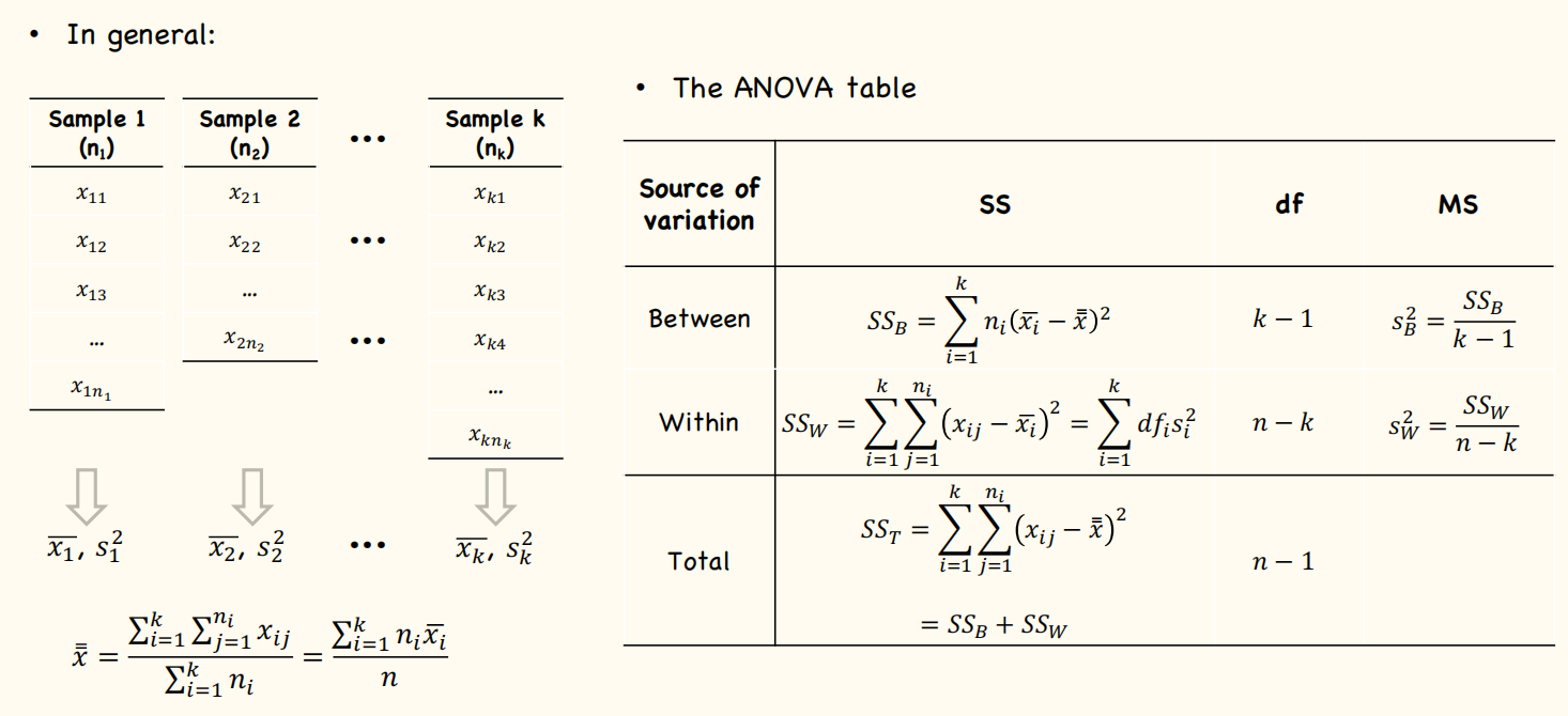
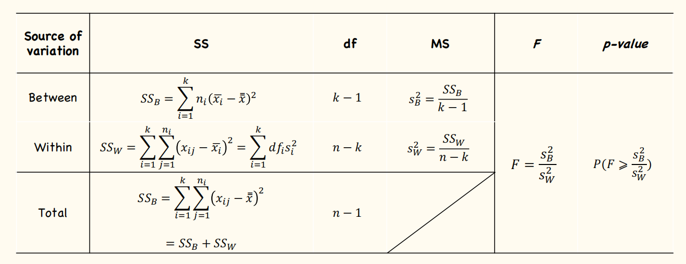
(1) Total sum of squares (SST)

$$
SS_{T} = \sum (x - \bar{\bar{x}})^2
$$

• $\bar{\bar{x}}$ is the grand mean, which is the mean of the whole sample space
• $x$ is each individual value in the whole sample space
• The degree of freedom: $df_{T} = n-1$, $n$ is the whole sample size

(2) Sum of squares within (SSW)

$$
SS_{W} = \sum (x_{1} - \overline{x_{1}})^2 + \sum(x_{2} - \overline{x_{2}})^2 + ··· + \sum(x_{k} - \overline{x_{k}} )^2 \
= df_{1} \cdot s_{1}^{2} + df_{2} \cdot s_{2}^{2} + ··· + df_{k}\cdot s_{k}^{2}
$$

• $k$ is the number of samples
• $x_{k}$ is each individual value in the $k^{th}$ sample, $\overline{x_{k}}$ is the mean of the $ k^{th}$ sample.
• $df_{k}$ is the degree of freedom of the $k^{th}$ sample where $df_{k} = \text{the sample size} - 1$, $s_{k}^{2}$ is the variance of the $k^{th}$ sample.
• $df_{W}$ = $\sum df_{k} = n-k$, n is the whole sample size

$$
s_{W}^{2} = \frac{SS_{W}}{n-k}
$$

(3) Sum of squares between (SSB)

$$
SS_{B} = \sum \Big{(} n_{k}\cdot (\overline{x_{k}} - \bar{\bar{x}})^2 \Big{)}
$$

• $k$ is the number of samples, $n_{k}$ is the sample size of each sample
• $\bar{\bar{x}}$ is the grand mean, which is the mean of the whole sample space
• $\overline{x_{k}}$ is the mean of the $ k^{th}$ sample.
• $df_{B} = k-1$

$$
s_{B}^{2} = \frac{SS_{B}}{k-1}
$$

(4) The ANOVA Table

F Test in ANOVA

$$
H_{0} : \mu_{1} = \mu_{2} = ··· = \mu_{k} \rarr F \leq 1\
H_{1} : \text{not all are equal} \rarr F > 1
$$

$$
F_{k-1, n-k} = \frac{S_{B}^{2}}{S_{W}^{2}}
$$

The p-value:
$$
\text{p-value} = P(\geq \frac{s_{B}^{2}}{s_{W}^{2}})
$$

Assumptions when using ANOVA

1. Randomness, independence
2. Population normally distributed
3. Variance:
   1. Different groups have equal variance (classical ANOVA) $\rarr s_{W}^{2} = \frac{SS_{W}}{n-k}$
   2. Unequal variance: Welch’s ANOVA

Post hoc tests

(1) Relationship between F-test and t-test

When there are only two groups: $F_{1,n-2} = t_{n-2}^{2}$

(2) Bonferroni Procedure

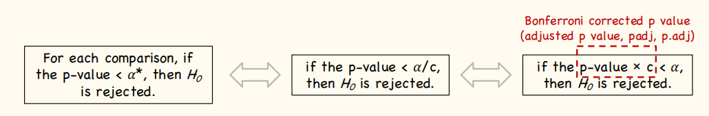
$$
\text{p.adj = min} \Big{[} p \times {k \choose 2} ,1 \Big{]}
$$
If $p.adj < \alpha$, then $H_{0}$ is rejected.

(3) Fisher’s Least Significant Difference (LSD)

Fisher’s LSD method is used in ANOVA to create confidence intervals for all pairwise differences between factor level means while controlling the individual error rate to a significance level you specify.

Therefore:
$$
t_{v} = \frac{(\bar{x}{1} - \bar{x}{2}) }{\sqrt{s_{p}^{2}(\frac{1}{n_{1}} + \frac{1}{n_{2}})}} \Rarr t_{v} = \frac{(\bar{x}{1} - \bar{x}{2}) }{\sqrt{s_{W}^{2}(\frac{1}{n_{1}} + \frac{1}{n_{2}})}}, v = n_{1}+n_{2} -2
$$

Chi-Square Test for Categorial Data

$$
\chi^2 = \sum_{cells} \frac{(O_{i} - E_{i})^2}{E_{i}}
$$

• $O_{i}$ is the observed data; $E_{i}$ is the expected data

$$
p = P(\chi_{v}^{2} \geq \chi^{2})
$$

• $v$ is t

2. 相关函数

aov

(1) 函数解释

在R中ANOVA可以通过函数aov()和lm()来实现。

• 虽然ANOVA和回归方法都是独立发展而来，但是从函数形式上看，它们都是广义线性模型的特例。讨论回归时用到的lm()函数也能分析ANOVA模型。

aov()的基本用法是：

aov(formula, data = NULL, projections = FALSE, qr = TRUE, contrasts = NULL, ...)

(2) 表达式（formula）

关于formula：

R表达式中常用的符号：

符号	描述
~	分隔符号，左边为响应变量，右边为解释变量。例如，要通过 x、z 和 w 预测 y，代码为 y ~ x + z + w
+	分隔预测变量
:	表示预测变量的交互项。例如，要通过 x、z 及 x 与 z 的交互项预测 y，代码为 y ~ x + z + x:z
*	表示所有可能交互项的简洁方式。代码 y~ x * z * w 可展开为 y ~ x + z + w + x:z + x:w + z:w + x:z:w
^	表示交互项达到某个次数。代码 y ~ (x + z + w)^2 可展开为 y ~ x + z + w + x:z + x:w + z:w
.	表示包含除因变量外的所有变量。例如，若一个数据框包含变量 x、y、z 和 w，代码 y ~ . 可展开为 y ~ x + z + w
-	减号，表示从等式中移除某个变量。例如，y ~ (x + z + w)^2 – x:w 可展开为 y ~ x + z + w + x:z + z:w
-1	删除截距项。例如，表达式 y ~ x - 1 拟合 y 在 x 上的回归，并强制直线通过原点
I()	从算术的角度来解释括号中的元素。例如，y ~ x + (z + w)^2 将展开为 y ~ x + z + w + z:w。 相反, 代码 y ~ x + I((z + w)^2)将展开为 y ~ x + h，h 是一个由 z 和 w 的平方和创建的新变量
function	可以在表达式中用的数学函数。例如，log(y) ~ x + z + w 表示通过 x、z 和 w 来预测 log(y)

常见研究设计的表达式:

描述	表达式
单因素 ANOVA	y ~ A
含单个协变量的单因素 ANCOVA	y ~ x + A
双因素 ANOVA	y ~ A * B
含两个协变量的双因素 ANCOVA	y ~ x1 + x2 + A*B
随机化区组	y ~ B + A （B 是区组因子）
单因素组内 ANOVA	y ~ A + Error(Subject/A)
含单个组内因子（W）和单个组间因子（B）的重复测量 ANOVA	y ~ B * W + Error(Subject/W)

• 小写字母表示定量变量，大写字母表示组别因子，Subject是对被试者独有的标识变量。

• 表达式中效应的顺序在两种情况下会造成影响：

  • 因子不止一个，并且是非平衡设计；

  • 存在协变量。出现任意一种情况时，等式右边的变量都与其他每个变量相关。

• 此时，我们无法清晰地划分它们对因变量的影响。例如，对于双因素方差分析，若不同处理方式中的观测数不同， 那么模型y ~ A*B与模型y ~ B*A的结果不同。

结果可视化

HH包中的ancova()函数可以绘制因变量、协变量和因子之间的关系图。

这部分演示使用multcomp包中的litter数据集进行演示：

> library(multcomp)
> head(litter)
  dose weight gesttime number
1    0  28.05     22.5     15
2    0  33.33     22.5     14
3    0  36.37     22.0     14
4    0  35.52     22.0     13
5    0  36.77     21.5     15
6    0  29.60     23.0      5

示例代码：

> library(HH)
> ancova(weight ~ gesttime + dose, data=litter)
Analysis of Variance Table

Response: weight
          Df  Sum Sq Mean Sq F value   Pr(>F)   
gesttime   1  134.30 134.304  8.0493 0.005971 **
dose       3  137.12  45.708  2.7394 0.049883 * 
Residuals 69 1151.27  16.685                    
---
Signif. codes:  0 ‘***’ 0.001 ‘**’ 0.01 ‘*’ 0.05 ‘.’ 0.1 ‘ ’ 1

3. 单因素方差分析 (ANOVA)

分析

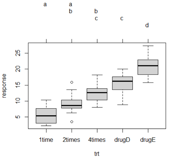
单因素方差分析中，你感兴趣的是比较分类因子定义的两个或多个组别中的因变量均值。以multcomp包中的cholesterol数据集为例:

> library(multcomp)
> attach(cholesterol)
> head(cholesterol)
    trt response
1 1time   3.8612
2 1time  10.3868
3 1time   5.9059
4 1time   3.0609
5 1time   7.7204
6 1time   2.7139

# 计算各组样本大小
# 每10个患者接受其中一个药物疗法
> table(trt)
trt
 1time 2times 4times  drugD  drugE 
    10     10     10     10     10 

# 计算各组均值
# 均值显示drugE降低胆固醇多，而1time降低胆固醇最少
> aggregate(response, by = list(trt), FUN = mean)
  Group.1        x
1   1time  5.78197
2  2times  9.22497
3  4times 12.37478
4   drugD 15.36117
5   drugE 20.94752

# 计算各组标准差
# 各组的标准差相对恒定，在2.88到3.48间浮动
> aggregate(response, by=list(trt), FUN=sd)
  Group.1        x
1   1time 2.878113
2  2times 3.483054
3  4times 2.923119
4   drugD 3.454636
5   drugE 3.345003

# 检验组间差异（ANOVA）
# ANOVA对治疗方式（trt）的F检验非常显著（p<0.0001），
# 说明五种疗法的效果不同
> fit <- aov(response ~ trt)

> fit
Call:
   aov(formula = response ~ trt)

Terms:
                      trt Residuals
Sum of Squares  1351.3690  468.7504
Deg. of Freedom         4        45

Residual standard error: 3.227488
Estimated effects may be unbalanced

> summary(fit)
            Df Sum Sq Mean Sq F value   Pr(>F)    
trt          4 1351.4   337.8   32.43 9.82e-13 ***
Residuals   45  468.8    10.4                     
---
Signif. codes:  0 ‘***’ 0.001 ‘**’ 0.01 ‘*’ 0.05 ‘.’ 0.1 ‘ ’ 1

# 展示数据：各组的均值和置信区间
> plot(response ~ trt)

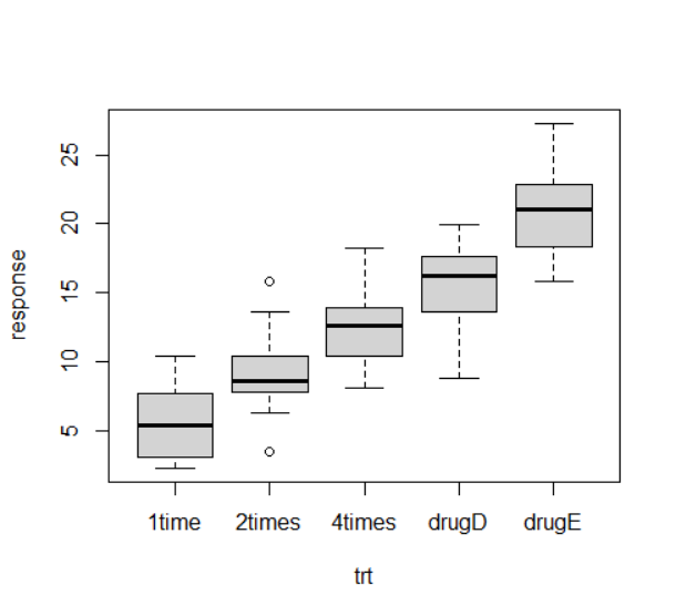
多重比较

虽然ANOVA对各疗法的F检验表明五种药物疗法效果不同，但是并没有告诉你哪种疗法与其他疗法不同。多重比较可以解决这个问题。例如，TukeyHSD()函数提供了对各组均值差异的成对检验，这个函数需要在aov()函数得到单因素方差分析的结果后（例如：fit <- aov(factor1 ~ factor2)），对得到的结果进行分析（例如: TukeyHSD(fit)，即TukeyHSD(aov(factor1 ~ factor2))）:

> ...

# 可以看到，1time和2times的均值差异不显著（p=0.138），
# 而1time和4times间的差异非常显著（p<0.001）。
> TukeyHSD(fit)
  Tukey multiple comparisons of means
    95% family-wise confidence level

Fit: aov(formula = response ~ trt)

$trt
                  diff        lwr       upr     p adj
2times-1time   3.44300 -0.6582817  7.544282 0.1380949
4times-1time   6.59281  2.4915283 10.694092 0.0003542
drugD-1time    9.57920  5.4779183 13.680482 0.0000003
drugE-1time   15.16555 11.0642683 19.266832 0.0000000
4times-2times  3.14981 -0.9514717  7.251092 0.2050382
drugD-2times   6.13620  2.0349183 10.237482 0.0009611
drugE-2times  11.72255  7.6212683 15.823832 0.0000000
drugD-4times   2.98639 -1.1148917  7.087672 0.2512446
drugE-4times   8.57274  4.4714583 12.674022 0.0000037
drugE-drugD    5.58635  1.4850683  9.687632 0.0030633

# 结果可视化
# 图形中置信区间包含0的疗法说明差异不显著（p>0.5）
> opar <- par()
> par(las = 2)
> par(mar=c(5,8,4,2))
> plot(TukeyHSD(fit))
> par(opar)

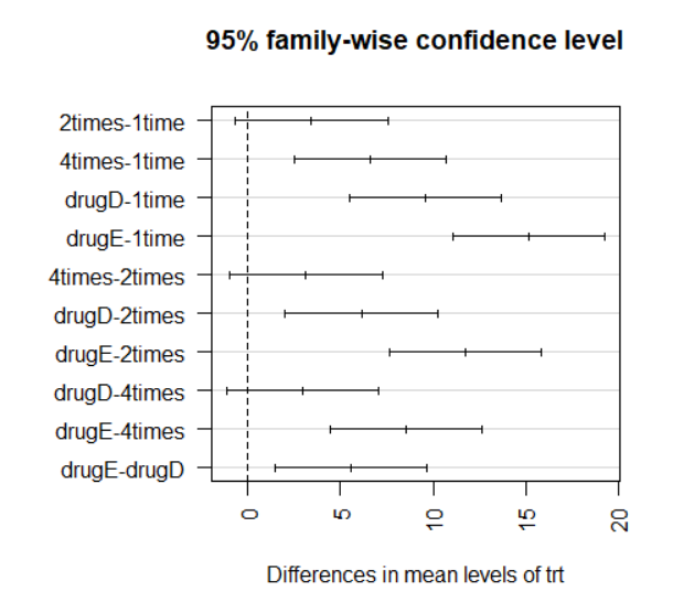
multcomp包中的glht()函数提供了多重均值比较更为全面的方法，既适用于线性模型，也适用于广义线性模型。

下面的代码重现了Tukey HSD检验:

> library(multcomp)

> tuk <- glht(fit, linfct=mcp(trt="Tukey"))
> tuk

	 General Linear Hypotheses

Multiple Comparisons of Means: Tukey Contrasts


Linear Hypotheses:
                     Estimate
2times - 1time == 0     3.443
4times - 1time == 0     6.593
drugD - 1time == 0      9.579
drugE - 1time == 0     15.166
4times - 2times == 0    3.150
drugD - 2times == 0     6.136
drugE - 2times == 0    11.723
drugD - 4times == 0     2.986
drugE - 4times == 0     8.573
drugE - drugD == 0      5.586

# 结果可视化
> opar <- par()
> par(mar=c(5,4,6,2))
> plot(cld(tuk, level=.05),col="lightgrey")
> par(opar)

评估检验的假设条件

我们对于结果的信心依赖于做统计检验时数据满足假设条件的程度。单因素方差分析中，我们假设因变量服从正态分布，各组方差相等。

这部分的演示使用multcomp包中的cholesterol来演示：

> data(cholesterol, package = "multcomp")
> head(cholesterol)
    trt response
1 1time   3.8612
2 1time  10.3868
3 1time   5.9059
4 1time   3.0609
5 1time   7.7204
6 1time   2.7139

(1) 正态性检验：Q-Q Plot

可以使用Q-Q图来检验正态性假设，这个过程需要使用car包中的qqPlot()函数：

示例代码：

> qqPlot(lm(response ~ trt, data=cholesterol), 
         simulate=TRUE, main="Q-Q Plot", labels=FALSE)
[1] 19 38

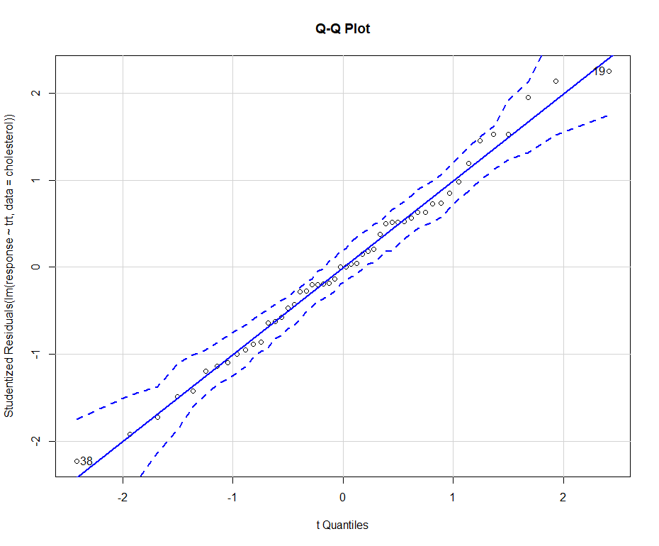
qqPlot()要求用lm()拟合。图形如上图所示。数据落在95%的置信区间范围内，说明满足正态性假设。

(2) 方差齐性检验

R提供了一些可用来做方差齐性检验的函数。例如，可以通过如下代码来做Bartlett检验：

> bartlett.test(response ~ trt, data=cholesterol)

	Bartlett test of homogeneity of variances

data:  response by trt
Bartlett's K-squared = 0.57975, df = 4, p-value = 0.9653

Fligner-Killeen检验（fligner.test()函数）:

> fligner.test(response ~ trt, data=cholesterol)

	Fligner-Killeen test of homogeneity of variances

data:  response by trt
Fligner-Killeen:med chi-squared = 0.74277, df = 4, p-value = 0.946

和Brown-Forsythe检验（HH包中的hov()函数）

> hov(response ~ trt, data=cholesterol)

	hov: Brown-Forsyth

data:  response
F = 0.075477, df:trt = 4, df:Residuals = 45, p-value = 0.9893
alternative hypothesis: variances are not identical

(3) 离群点检测

可利用car包中的outlierTest()函数来检测离群点：

> library(car)
> outlierTest(fit)
No Studentized residuals with Bonferroni p < 0.05
Largest |rstudent|:
    rstudent unadjusted p-value Bonferroni p
63 -3.109569          0.0027364       0.2025

---

对于这个例子，综上：从输出结果来看，并没有证据说明胆固醇数据（cholesterol）中含有离群点（当p>1时将产生NA）。因此根据Q-Q图、Bartlett检验和离群点检验，该数据似乎可以用ANOVA模型拟合得很好。这些方法反过来增强了我们对于所得结果的信心。

4. 单因素协方差分析 (ANCOVA)

计算

单因素协方差分析（ANCOVA）扩展了单因素方差分析（ANOVA），包含一个或多个定量的协变量。

这部分演示使用multcomp包中的litter数据集进行演示：

> data(litter, package = "multcomp")
> head(litter)
  dose weight gesttime number
1    0  28.05     22.5     15
2    0  33.33     22.5     14
3    0  36.37     22.0     14
4    0  35.52     22.0     13
5    0  36.77     21.5     15
6    0  29.60     23.0      5

示例代码：

> attach(litter)

> table(dose)
dose
  0   5  50 500 
 20  19  18  17 

> aggregate(weight, by=list(dose), FUN=mean)
  Group.1        x
1       0 32.30850
2       5 29.30842
3      50 29.86611
4     500 29.64647

> fit <- aov(weight ~ gesttime + dose)
> summary(fit)
            Df Sum Sq Mean Sq F value  Pr(>F)   
gesttime     1  134.3  134.30   8.049 0.00597 **
dose         3  137.1   45.71   2.739 0.04988 * 
Residuals   69 1151.3   16.69                   
---
Signif. codes:  0 ‘***’ 0.001 ‘**’ 0.01 ‘*’ 0.05 ‘.’ 0.1 ‘ ’ 1

> detach(litter)

计算调整的均值

由于使用了协变量，你可能想要获取调整的组均值，即去除协变量效应后的组均值。可使用effects包中的effects()函数来计算调整的均值：

> library(effects)

> effect("dose", fit)

 dose effect
dose
       0        5       50      500 
32.35367 28.87672 30.56614 29.33460 

多重比较

使用multcomp包来对所有均值进行成对比较。另外，multcomp包还可以用来检验用户自定义的均值假设。

> library(multcomp) 
> contrast <- rbind("no drug vs. drug" = c(3, -1, -1, -1)) 
> summary(glht(fit, linfct=mcp(dose=contrast)))

	 Simultaneous Tests for General Linear Hypotheses

Multiple Comparisons of Means: User-defined Contrasts


Fit: aov(formula = weight ~ gesttime + dose)

Linear Hypotheses:
                      Estimate Std. Error t value Pr(>|t|)  
no drug vs. drug == 0    8.284      3.209   2.581    0.012 *
---
Signif. codes:  0 ‘***’ 0.001 ‘**’ 0.01 ‘*’ 0.05 ‘.’ 0.1 ‘ ’ 1
(Adjusted p values reported -- single-step method)

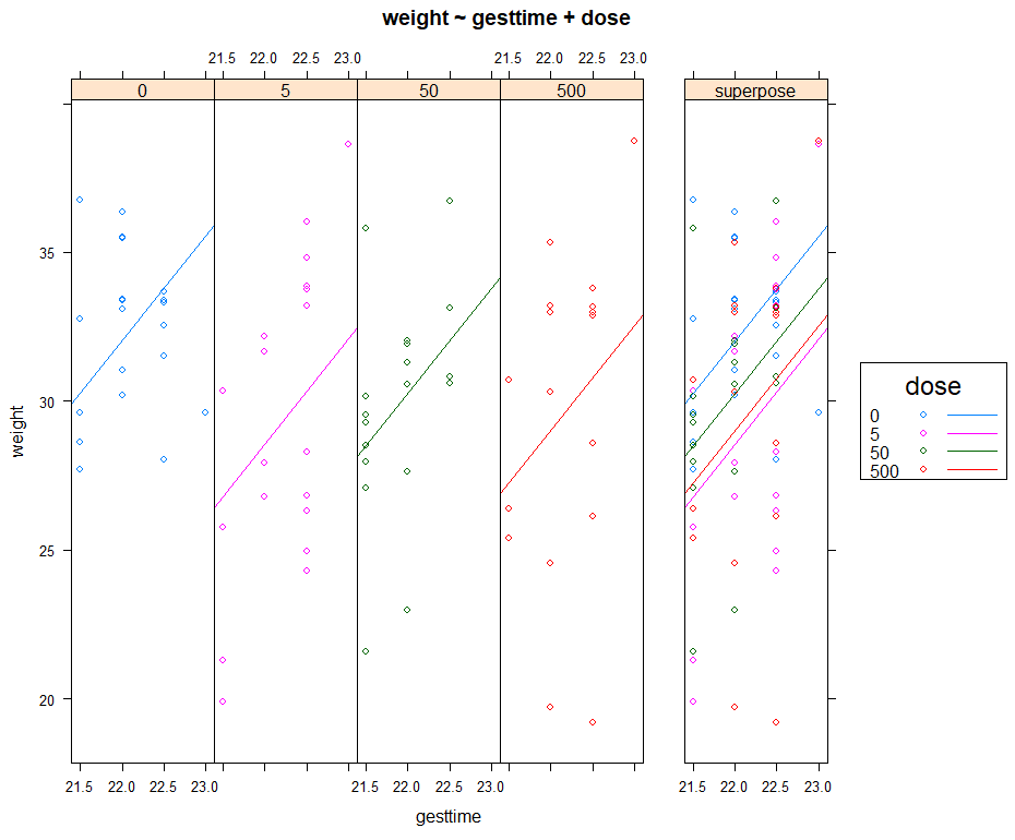
评估检验的假设条件: ANCOVA Special，检验回归斜率的同质性

ANCOVA与ANOVA相同，都需要正态性和同方差性假设，可以用在ANOVA中提到的相同的步骤来检验这些假设条件。另外，ANCOVA还假定回归斜率相同。

以multcomp包中的litter数据集为例：

> head(litter)
  dose weight gesttime number
1    0  28.05     22.5     15
2    0  33.33     22.5     14
3    0  36.37     22.0     14
4    0  35.52     22.0     13
5    0  36.77     21.5     15
6    0  29.60     23.0      5

假定四个处理组通过怀孕时间 (gesttime)来预测出生体重 (weight)的回归斜率都相同。ANCOVA模型包含怀孕时间 (gesttime)×剂量 (dose)的交互项时，可对回归斜率的同质性进行检验。交互效应若显著，则意味着时间和幼崽出生体重间的关系依赖于药物剂量的水平：

> library(multcomp) 
> fit2 <- aov(weight ~ gesttime*dose, data=litter) 
> summary(fit2)
              Df Sum Sq Mean Sq F value  Pr(>F)   
gesttime       1  134.3  134.30   8.289 0.00537 **
dose           3  137.1   45.71   2.821 0.04556 * 
gesttime:dose  3   81.9   27.29   1.684 0.17889   
Residuals     66 1069.4   16.20                   
---
Signif. codes:  0 ‘***’ 0.001 ‘**’ 0.01 ‘*’ 0.05 ‘.’ 0.1 ‘ ’ 1

可以看到交互效应不显著，支持了斜率相等的假设。若假设不成立，可以尝试变换协变量或因变量，或使用能对每个斜率独立解释的模型，或使用不需要假设回归斜率同质性的非参数ANCOVA方法。sm包中的sm.ancova()函数为后者提供了一个例子。

---

方差分析当然不止这么点，只不过双因素方差分析、重复测量方差分析、多元方差分析对我来说用的实在太少，于是也就不费心在这里去记录课本上的内容以及相关笔记了。